Chapter 1 Introduction

Welcome to this course on algorithms and programming! This course is about programming, of course, but it is also about problem-solving. If there’s one thing that you take away from this course, it should be that computer science is about the science of solving problems — the fact that we use computers to do this is efficient, but actually besides the point.

Throughout this book, you will see two kinds of question boxes from time to time:

Question! This is a question box that will test you have understood the concepts presented in the notes. I recommend tackling the questions to make sure you have a good understanding before moving on.

Side quest! This is a “side quest” box. These are random questions, tasks and digressions that you may wish to look into if you are curious. They are not necessary, but are just fun activities that you may be interested in tackling. Learning shouldn’t be about doing something because you have to.

We will be using multiple programming languages in this course. The key takeaway here is that languages are just tools to get the computer to do what we want it to. The core fundamentals of programming (and problem-solving) are the same, regardless of the language we use. That is why this course is not called “Introduction to Programming with Python.” In this chapter we will discuss the core elements of problem-solving (algorithms), and then move onto how we can actually get the computer to do the work for us (programming).

1.1 Algorithms

The first question we might ask is: what exactly is an algorithm? Informally, we can think of an algorithm as a solution to a problem. However, an algorithm is no ordinary solution — an algorithm is a solution that is so complete, it can solve any instantiation of the given problem.

To illustrate what we mean by this, let’s consider the following example. We’re walking down the street and a young kid approaches us The conversation goes as follows:

Kid: Excuse me, but can you help me?
Us: Sure, what’s wrong?
Kid: We’re learning about even and odd numbers in school! 
     Can you please tell me all the even numbers from 1 to 10?
Us: Sure, the even numbers are 2, 4, 6, 8, 10!
Kid: Thanks! You’re so smart! Bye now!

Okay, so in this example we were given a problem and we able to provide a solution. No problem! But now imagine the kid is a bit of a smarty-pants, and instead asks the following question:

Kid: Can you please tell me all the even numbers from X to Y?
Us: Sure, but it depends. What is X and Y?
Kid: I don’t know. I haven’t decided yet.
Us: …

Well now we have a bit of a problem. We could claim that we can’t give an answer until the kid tells us the values of \(X\) and \(Y\), but then we wouldn’t seem very smart, and the kid would run home and tell his parents how the grown-ups are all stupid! So what else can we do? How can we answer such an open question?

Then we hit on an idea. Instead of giving the kid a direct answer (which is impossible), we can give him instructions on how to find the correct answer once he’s decided what the values of \(X\) and \(Y\) are! Our conversation could go something like:

Us: Sure, but it depends. What is X and Y?
Kid: I don’t know. I haven’t decided yet.
Us: Okay, well in that case, here’s what you 
    do when you eventually decide what X and Y are.
    If X is divisible by 2 (let’s assume for now he
    knows what divisible means), then the first even 
    number is X, the second number is X+2, and you 
    keep adding 2 until you get to a number bigger 
    than Y, at which point you stop. However, if X 
    is not divisible by 2, then the first even number
    is X+1, the second even number is X+3, and then 
    you keep going up in steps of 2 until you get to
    a number bigger than Y, at which point you stop.

Satisfied, the kid runs off and tell his parents how smart we are!

What we have done here is provided an answer to the problem as a sequence of instructions. Informally, this is what we would call an algorithm. Note that our solution is completely general! We can plug in any values for \(X\) and \(Y\), and if we follow our instructions, we’ll get the right answer!

This is the magical thing about algorithms and computer science in general — it’s not about solving one particular problem, it’s about solving all instances of a particular problem class! Think of this like making the step from arithmetic to algebra in school, but instead of mathematics, we’re solving problems! For example, maybe you enjoy doing crosswords? In that case, you could develop an algorithm (with some difficulty) for solving not just the crossword you’re currently working on, but any crossword! The same for chess: let’s not just solve a particular position, let’s solve any position! Sudoku? Let’s solve all the Sudokus! You get the point.

1.1.1 The Science of Problems

At its heart, theoretical computer science deals with issues like: What makes one problem harder or more difficult than another? Can we quantify what we mean by “difficult?” A natural response to these questions might be to wonder: doesn’t it depend on the person solving the problem? For example, we might find solving a quadratic equation straightforward, but someone who has never done mathematics will find it impossible!

As it turns out, the question of difficulty has nothing to do with the solver — it is all about the fundamental properties of the problem itself!

Philosophy side quest! Think about the implications of the fact that certain problems are just intrinsically harder than others, no matter how smart you are or how many people are working on it! For example, a major open question is: is solving a hard problem more difficult that verify that the solution is in fact correct? This is what is known as the classic \(P \neq NP?\) problem. Most theoreticians believe this to be true, but we have yet to prove this. This would be equivalent to saying: it is much harder to create a work of art than it is to verify that the object is in fact art. What would it mean if this were not the case?!

Let’s look at an example to make this concrete.

Problem 1: What is \(x \times y\) where \(x =\) 33478071698956898786044169848212690817704794983713768568912431388982883793878002287614711652531743087737814467999489 and \(y=\) 36746043666799590428244633799627952632279158164343087642676032283815739666511279233373417143396810270092798736308917?

Problem 2: Find two positive integers \(x\) and \(y\), both greater than \(1\), so that \(x \times y=\) 2519590847565789349402718324004839857142928212620403202777713783604366202070 7595556264018525880784406918290641249515082189298559149176184502808489120072 8449926873928072877767359714183472702618963750149718246911650776133798590957 0009733045974880842840179742910064245869181719511874612151517265463228221686 9987549182422433637259085141865462043576798423387184774447920739934236584823 8242811981638150106748104516603773060562016196762561338441436038339044149526 3443219011465754445417842402092461651572335077870774981712577246796292638635 6373289912154831438167899885040445364023527381951378636564391212010397122822120720357

Which problem do you think is harder? The first one may look like a tough multiplication problem, but it is actually relatively straightforward given enough patience. A ten year old with sufficient concentration could solve it! The second problem, which seems very related to the first, is really hard. In fact, it is so hard, that no man or computer has ever discovered the answer. It is so hard (and provably so) that you would win ONE MILLION DOLLARS for coming up with the solution! It is so hard that every sensitive piece of information ever produced — your bank details, your passwords, nuclear missile launch codes — relies on the fact that the problem cannot be solved in any reasonable amount of time. And yet it seems so related to the first problem, that it should be simple. So why isn’t it?! It’s these kinds of questions that computer science, at its core, deals with.

1.1.2 Properties of an Algorithm

We have so far only informally referred to an algorithm as a set of instructions that forms a solution to a particular problem. But let’s be a bit more specific.

An algorithm is a set of well-defined, unambiguous steps or instructions to be carried out in sequence to accomplish some task. Note here that the instructions must be precise and exact. There must be no room for interpretation or confusion!
An algorithm is made up of individual instructions.
There can only be a finite set of instructions – no infinity please!
Each instruction is well-defined and its outcome predictable if the instruction operates on valid input
An algorithm has a start and stop point. The start may require some inputs, and the stop may provide some output.
There is a direction of logic flow or sequencing. Once an instruction is executed, it passes control to another instruction.
When executed (with valid input) an algorithm is guaranteed to terminate in a sensible way.

Question! Based on these properties, consider the statements below and decide whether they are in fact algorithms. If not, why not?

Add some numbers from 1 to 10.
Add up all the natural numbers from 1 to 10 (inclusive).
Add up all the natural numbers.
Add up all the real numbers from 0 to 1.

Mathematics side quest!

Are there more real numbers between 0 and 1 than there are natural numbers?
Are there more real numbers between 0 and 2 than there are real numbers between 0 and 1?
Are there more real numbers than there are real numbers between 0 and 1?

Having seen the properties of an algorithm, let’s look at an example and see how we would read and follow it:

The above representation is known as pseudocode. As you can see, it is an artificial informal language that mixes mathematics and English. There are no standard rules for putting pseudocode together, but it can be used to help us ‘’think out’’ a solution to a problem! Another representation you may come across is a flowchart, which is simply a graphical representation of an algorithm, but we won’t go into those here.

1.2 Programming

You may have noticed that at this point we have made no mention of computers or programming even once! So what’s the link between the two? Well, once we’ve come up with a solution to a problem in the form of an algorithm, the question is: who is going to execute the sequence of instructions? I mean, we could do it, but that would be time-consuming (especially if there are millions of instructions), and we have better things to do. So instead, we’re going to get a computer to execute it for us! Computers don’t get tired, they don’t need to eat, and they really have nothing else to do — the perfect candidates for the job! Programming is nothing more than turning an algorithm into something a computer can understand and execute. An algorithm that has been turned into something executable by a computer is known as a program. Before we get into programming, let’s talk about what computer are and are not.

1.2.1 A Brief History of Modern Computers

The first computers were the women employees of the JPL lab in 1936. They were known as the NASA human computers and their job was to perform calculations on pen and paper every day, the results of which were ultimately used by NASA to launch their space shuttles!

History side quest! Watch the 2016 film Hidden Figures.

The very first instance of what we would now refer to as a computer was built in 1945. It was called the ENIAC (Electronic Numerical Integrator and Computer) — it weighed 30 000kg and took up 167\(m^2\) of space. It could perform an astounding three hundred and fifty seven multiplication operations per second, clearly much faster than any human could ever hope to achieve. (For reference, your cellphone can perform well over a billion operations per second).

ENIAC’s first task was to compute whether or not it was possible to build a hydrogen bomb (the bomb had already been constructed at this point, so this was just a test). The very first problem run on ENIAC required only 20 seconds and was checked against an answer obtained after forty hours of work with a mechanical calculator. The entire program was encoded on more than half a million punch cards, and after six weeks, ENIAC produced output declaring the hydrogen bomb feasible. This first ENIAC program remains classified to this day

1.2.2 Doing Arithmetic with Electricity

How a computer works and executes operations is the topic of another course, but let’s briefly explain how we instruct computers. Computers are made up of electronic circuits that perform addition and various other mathematical operators. The question then is: how do we represent numbers with electricity? Well, we really have only two options. Either there is electricity present, or there isn’t. We might think of these as representing the numbers \(1\) and \(0\). \(1\) for electricity on. \(0\) for electricity off. But how does this help us represent numbers if we only have \(0\) and \(1\)?

To answer this, let’s think about the numbers we use — we work in decimal numbers, which means we have the symbols \(0\)–\(9\) that can be combined to produce any number we want. But why are there ten symbols? There’s no real reason (probably because we have ten fingers). It’s completely arbitrary! We could have 9 symbols, or 12 symbols or 32 symbols, or we could replace the digits with hieroglyphics. It doesn’t really matter because…

Figure 1.1: Right on, Mr Incredible!

As you will see in BCO, one particularly important number system is binary, consisting of only two symbols: \(0\) and \(1\). And we can use these to represent any number we care about. For example:

Decimal number	Binary number
0	00000000
1	00000001
2	00000010
3	00000011
4	00000100
5	00000101
6	00000110
7	00000111
8	00001000

And so on (do you notice the pattern?).

1.2.3 Programming languages

So at the very lowest level, computers execute mathematical operations using ones and zeros. Should we instruct computers this way? Well, at first we had to. There was no other choice. However, we soon realised that this was really tough and annoying. Typing ones and zeros all day is slow going, and it’s really easy to make a mistake.

To overcome this, we developed a programming language. We would write some text in human-readable manner, and this would be directly converted into 1s and 0s. This is known as assembly and is still used today for low-level programming. We can think of assembly as looking something like this that maps text to binary numbers:

LOAD PAY     -> 01010001
ADD OVERTIME -> 10110101
STORE TOTAL  -> 00000001

But very soon, even assembly became tiresome. You have to write a lot of code to do some very simple things. Furthermore, it was architecture-dependent. Assembly for Windows would not work on a Mac or on Ubuntu, for example. The solution, of course, is simply to create a higher-level language, creating a hierarchy of increasingly abstract programming languages. The programmer would write their code in the high-level language, which would then be converted into assembly, which would ultimately be converted into ones and zeros. We can continue this trend infinitely, creating more and more languages that are built on top of one another! Of course, programming languages are just tools to get the job done, so if you need a high-level programming language, then you should use one. But if you need to program a washing machine, for example, then assembly is probably your best choice.

1.2.4 Compiled and Interpreted Languages

Broadly speaking, there are two classes of languages (although some will blur the lines): compiled and interpreted. In the first half of this course we will be using Python, an interpreted language, while in the second half we will use C++, which is compiled.

The difference between the two can be illustrated by this example. Imagine we are asked to give a speech to a group of politicians from Spain. Unfortunately, we don’t speak Spanish, so what can we do? Fortunately, we don’t actually have to present the speech ourselves, so we can hire someone who speaks English and Spanish, give him our speech that we’ve written in English, and go from there. Let’s look at the compiled vs interpreted way of doing this.

The Compiled Way: We write our speech in English. The day before, we hand it to our employee who then translates the speech into Spanish and writes it down. The next day, we send him to the presentation and he reads the speech out. Success!

The Interpreted Way: We write our speech in English. On the day of the presentation, we go with our employee to the meeting. He stands at the microphone and we whisper the first line to him in English. He translates it on the spot and announces the first line in Spanish. Then we whisper the second line. He translates it for the audience. Then we do the third line, and so on!

In a programming context, a compiled language comes with a program known as a compiler. This compiler is architecture specific, so a compiled language must have a compiler for Windows, and another for MacOS, and so on. This compiler accepts a high-level language as input and outputs a low-level (machine code) language. This low-level language can then be directly run on the computer. Every time we wish to run the program, we can just directly execute the low-level code — no translation needs to occur.

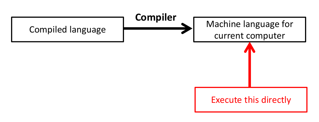
Figure 1.2: Our code is compiled and converted into machine code. When we want to run the program, we just execute this machine code directly.

An interpreted language comes with a special program known as the interpreter. The programmer writes the program in a high-level language, and this is fed into the interpreter one line at a time! The first line is translated into machine code and then executed on the computer, then the second line is translated, and so on. Every time we execute the program again, this translation occurs!

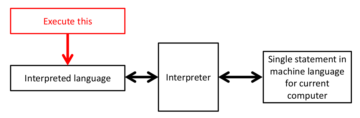
Figure 1.3: Our code is translated and executed one line at a time. Every time we want to run the code, we have to go through this translation process.

Which way is better? Well, the first seems much more realistic and faster! Who would bother with the second way?! It turns out, both approaches have merits and downsides. Clearly the first way is quicker: we only need to translate the code once! However, the interpreted way also has some advantages – the high-level language code is available (since it needs to be run) which promotes openness, and the code can quickly be edited and changed on the fly. In the compiled case, once the low-level language is produced, it’s almost impossible to make changes to it!

Question! Head to our favourite place (Google) and make a list of some of the pros and cons of using an interpreted or compiled language.

1.2.5 A Quick Look at Python

We will now briefly look at Python, the interpreted language we’ll be focusing on. In particular, we wil be using Python 3, the third version of the language (note that your Python version number might look like 3.X.X — as long as it starts with a 3, you’re all good). When programming (with whatever the language), there are two aspects to it. The first is writing the code – we do this by typing the high-level language in a text file. The next step is executing the code, which in the case of Python, we do using the interpreter. In the video below, we show how to do this in Ubuntu.

The video below shows how to execute Python code using the Windows operating system and IDLE.