Chapter 2 Differential Equations

“Among all of the mathematical disciplines the theory of differential equations is the most important… It furnishes the explanation of all those elementary manifestations of nature which involve time.” - Sophus Lie (1842-1899)

2.1 Differential Equations and Ordinary Differential Equations

Before we formally construct and solve any continuous models in Chapter 3, we will be unpacking what an ordinary differential equation is, the ways in which we can classify them, and hence the methods of solution we can adopt in order to find analytical solutions. It will be useful at this juncture to discuss some useful definitions.

Remark. At this stage, I want to emphasize that you are registered for a degree in the mathematical sciences. You should not be afraid to grapple with technical and theoretical mathematical definitions. It is a key toolkit within your arsenal that you need to develop. If you have discomfort trying to decipher a mathematical definition, that is okay. However, you need not shy away from doing so, but instead try to make meaning that links the theory to the concepts There is an inherent discomfort to learning. You also need to develop an aptitude for reading with comprehension. Spoiler: If you thought there was a lot of reading to do last week, wait until Chapter 3. *rant over*

Definition 2.1 (Differential Equation) A differential equation (DE) is a mathematical equation that relates a function with its derivatives.

Definition 2.2 (Ordinary Differential Equation) An ordinary differential equation (ODE) is an equation that involves some ordinary derivatives of one or more unknown function (the dependent variable(s)) of one single independent variable.

For example: \[\begin{equation} \dfrac{d^2 y}{dx^2}+3\dfrac{d y}{dx}+2y=\sin{x} \tag{2.1} \end{equation}\]

Definition 2.3 (Partial Differential Equation) In contrast, a partial differential equation is an equation that involves some partial derivatives of one or more unknown function (the dependent variable(s)) of two or more independent variables.

For example: \[\begin{equation} \dfrac{\partial^2 u}{\partial x^2}+ \dfrac{\partial^2 u}{\partial y^2}=0 \end{equation}\]

The work we do will do regarding differential equations in this course will exclusively involve ordinary differential equations. This means that we will have only one independent variable. For the rest of these notes, any reference to the word differential equation and the abbreviation DE refers exclusively to ordinary differential equations You will consider partial differential equations in subsequent years, once you have a firmer grasp of multivariable calculus.

Differential equations arise from many sources, and the independent variable can signify many different things. In these notes we will use a variety of variables for for the independent variable (including time \(t\)), likewise for the dependent variable (excluding time \(t\)). Nonetheless, very often the independent variable represents time, and the dependent variable is some dynamical quantity which depends upon time.

2.2 Notation

Throughout these notes, ordinary derivatives will be denoted with the use of either the Leibniz notation, the prime notation, or Newton’s dot notation.

Update: Newton’s dot notation is most commonly used in physics, and it is mostly, but not exclusively, used to represent change with respect to time \(t\).

2.3 Classification of an Ordinary Differential Equation

Consider the the general ordinary differential equation given below,

\[\begin{equation} a_{n}(x)\dfrac{d^n y}{dx^n}+a_{n-1}(x)\dfrac{d^{n-1} y}{dx^{n-1}}+\dots+ a_{2}(x)\dfrac{d^2 y}{dx^2}+a_{1}(x)\dfrac{d y}{dx}+a_{0}(x)y=g(x) \tag{2.2} \end{equation}\] where the coefficient functions, \(a_{n}(x), a_{n-1}(x), \dots, a_{2}(x), a_{1}(x), g(x)\) can be any functions of the independent variable \(x\) (including a constant/zero function).

We are interested in distinguishing all resultant ODEs that can be extracted from the above general ODE from each other by considering some of its constituent features. There are many ways to relate a function with its derivatives. When this is done, we find the following classifications of an ODE useful:

2.3.1 Order

2.3.2 Linearity

2.3.3 Homogeneity

2.3.4 Coefficients

Remark. One of the reasons we are interested in doing so is that once we are able to classify certain ordinary differential equations using the above features, it will give us better insights into what solution methods and procedures are best suited to deploy in order to solve that particular differential equation. At this stage, it may seem unneccesary, but you will see the importance of doing so in later sections within this chapter.

2.3.1 Classification by order

Definition 2.4 (Order of an Ordinary Differential Equation) The order of a differential equation is the order of the highest derivative in the differential equation.

The order of Equation (2.1) is \(2\) or it is of the \(2\)nd order. This corresponds to the term with the highest derivative operator \(\dfrac{d^2 y}{dx^2}\).

The order of Equation (2.2) is \(n\) or it is of the \(n\)th order. This corresponds to the term with the highest derivative operator \(\dfrac{d^n y}{dx^n}\).

2.3.2 Classification by linearity

Definition 2.5 (Linearity of an Ordinary Differential Equation) A linear differential equation is one in which neither the unknown function nor any of its derivatives are raised to a power greater than 1.

An \(nth\)-order ODE such as in Equation (2.2) is said to be linear if

• the dependent variable (in this case, \(y\)) and all of its derivatives are of the first degree, that is, the power of each term involving the dependent variable \(y\) is 1, and
• the coefficients of the dependent variable \(y\) and any of its derivatives are constants, or they depend on the independent variable (in this case, \(x\)) only.

A differential equation that is not linear is said to be non-linear and this occurs when the above does not hold, that is, non-linear functions of the dependent variable or any of its derivatives occur in the differential equation.

Equation (2.1) is linear as \(\dfrac{d^2 y}{dx^2}, \dfrac{d y}{dx},\) and \(y\) are of the first degree, and its coefficients are all constants (1, 3, and 2 respectively). \(\sin{x}\) is non-linear in the independent variable, and thus has no effect on the linearity of Equation (2.1).

2.3.3 Classification by homogeneity

Definition 2.6 (Homogeneity of an Ordinary Differential Equation) A differential equation is homogeneous with respect to the dependent variable (say \(y\), in this case) if replacing the dependent variable with a non-zero arbitrary constant multiplied by the dependent variable does not change the structure of the differential equation. We say that the differential equation remains invariant under this transformation.

Otherwise, the differential equation is said to be non-homogeneous with respect to the dependent variable (in this case, \(y\)).

Otherwise stated, the ODE is homogeneous in the dependent variable if the substitution of \(ky\) (where \(k\) \(\neq\) 0) for \(y\) in the differential equation does not change the ODE. We will refer to this as the test for homogeneity. Any ODE that changes upon implementing the test will be classified as non-homogeneous.

We now implement the test for homogeneity on Equation (2.1) to check if this equation is homogeneous or not. To do this, let \(y=ky\), and so Equation (2.1) becomes \[\begin{equation} \dfrac{d^2 (ky)}{dx^2}+3\dfrac{d (ky)}{dx}+2ky=\sin{x}, \end{equation}\] \[\begin{equation} k\dfrac{d^2 y}{dx^2}+3k\dfrac{d y}{dx}+2ky=\sin{x}, \end{equation}\] \[\begin{equation} k\left( \dfrac{d^2 y}{dx^2}+3\dfrac{d y}{dx}+2y\right) =\sin{x}, \end{equation}\] \[\begin{equation} \dfrac{d^2 y}{dx^2}+3\dfrac{d y}{dx}+2y=\frac{1}{k}\sin{x}. \tag{2.3} \end{equation}\] Recall that \(k\) is a non-zero constant, i.e. \(k\neq 0.\) Thus, we can conclude that Equation (2.1) is non-homogeneous as the structure of the original Equation (2.1) and the resultant transformed Equation (2.3) are different.

Now, let us remove \(\sin{x}\) in Equation (2.1) to get the equation \[\begin{equation} \dfrac{d^2 y}{dx^2}+3\dfrac{d y}{dx}+2y=0. \tag{2.4} \end{equation}\] Let us now conduct the test for homogeneity on Equation (2.4). Again we let \(y=ky\) to get, \[\begin{equation} \dfrac{d^2 (ky)}{dx^2}+3\dfrac{d (ky)}{dx}+2ky=0, \end{equation}\] \[\begin{equation} k\dfrac{d^2 y}{dx^2}+3k\dfrac{d y}{dx}+2ky=0, \end{equation}\] \[\begin{equation} k\left( \dfrac{d^2 y}{dx^2}+3\dfrac{d y}{dx}+2y\right) =0, \end{equation}\] Since \(k \neq 0\), it follows that \[\begin{equation} \dfrac{d^2 y}{dx^2}+3\dfrac{d y}{dx}+2y=0 \tag{2.5} \end{equation}\] Equation (2.4) is homogeneous as it is the same as Equation (2.5) under the transformation, i.e. the equation remained invariant.

Let us now clarify or refine this definition for homogeneity for linear ordinary differential equations.

Definition 2.7 (Homogeneity of a Linear Ordinary Differential Equation) Consider the \(nth\)-order linear ODE given in Equation (2.2). \[\begin{equation} a_{n}(x)\dfrac{d^n y}{dx^n}+a_{n-1}(x)\dfrac{d^{n-1} y}{dx^{n-1}}+\dots+ a_{2}(x)\dfrac{d^2 y}{dx^2}+a_{1}(x)\dfrac{d y}{dx}+a_{0}(x)y=g(x) \tag{2.2} \end{equation}\] where the coefficient functions, \(a_{n}(x), a_{n-1}(x), \dots, a_{2}(x), a_{1}(x), g(x)\) can be any functions of the independent variable \(x\) (including a constant/zero function).

Equation (2.2) is non-homogeneous with respect to the dependent variable (say \(y\), in this case) if \(g(x) \neq 0\), in other words \(g(x)\) is not identically zero and the ODE contains terms that are functions of the independent variable, including constants.

Now consider the case when \(g(x)=0\), that is \[\begin{equation} a_{n}(x)\dfrac{d^n y}{dx^n}+a_{n-1}(x)\dfrac{d^{n-1} y}{dx^{n-1}}+\dots+ a_{2}(x)\dfrac{d^2 y}{dx^2}+a_{1}(x)\dfrac{d y}{dx}+a_{0}(x)y=0 \tag{2.6} \end{equation}\] An \(nth\)-order linear ODE such as in Equation (2.6) is homogeneous with respect to the dependent variable (say \(y\), in this case) if \(g(x)=0\), in other words it does not contain any term that is a function of the independent variable only, including constants.

Based on the above refined definition for homogeneity for linear ODEs, Equation (2.1) is a non-homogeneous second-order linear ordinary differential equation since \(g(x)=\sin x\) (a non-zero function of the independent variable \(x\)), whereas Equation (2.4) is a homogeneous second-order linear ordinary differential equation since \(g(x)=0\).

Remark. One can only use Definition 2.7 for homogeneity once you have concluded that the ODE is linear. In that case, homogeneity can be done by inspection based on whether the function of the independent variable \(g(x)=0\) (homogeneous) or \(g(x) \neq 0\) (non-homogeneous).

To summarize: the key difference between homogeneous and non-homogeneous linear ODEs is the presence of a forcing term. In a non-homogeneous linear ODE, there is an additional term which is not identically zero: a function (on the right-hand side) that depends on the independent variable, such as \(f(x)\) or \(g(t)\). This function is called the forcing term or the non-homogeneous part of the equation because it forces the solution to have a particular behaviour. Non-homogeneous ODEs are used to model phenomena where there is an external influence on the system being modeled, such as in electrical circuits or mechanical systems.

In contrast, a homogeneous linear ODE is an equation in which the forcing term is identically zero. Homogeneous ODEs are used to model phenomena where the system being modeled is self-contained and does not have any external influences. An example of a homogeneous ODE is \(y'' + 4y' + 3y = 0\), where \(y=y(x)\), which models the behavior of a mass-spring system without any external forces acting on it.

2.3.4 Classification by coefficients

Definition 2.8 (Coefficients of an Ordinary Differential Equation) The coefficient of any term of an ODE is that factor of the term which does not involve the unknown function or any of its derivatives. An ODE can have constant or variable (non-constant) coefficients.

An ODE has constant coefficients if all terms in the equation involving the dependent variable and its derivatives are preceded by coefficients that are constants.

An ODE has variable coefficients if at least one of the terms in the equation involving the dependent variable and its derivatives are preceded by coefficients that are functions of the independent variable.

Equation (2.1) has constant coefficients. The coefficients of \(\dfrac{d^2 y}{dx^2}\) is 1, \(\dfrac{d y}{dx}\) is 3, and \(y\) is 2, all of which are constants.

The coefficients play a crucial role in determining the behavior of the solution to an ODE. They can affect whether the solution is oscillatory or decaying, and they can also impact the stability of the solution. Understanding the coefficients is essential for solving and interpreting ODEs.

Classification of Differential Equations: Examples

1. \(\dfrac{d^2 y}{dx^2}-2\dfrac{d y}{dx}+3y=0\)

2. \(5 \dfrac{d^2 x}{dt^2}+7\dfrac{d x}{dt}-8x=e^{x}\)

3. \(x^2\dfrac{d^2 y}{dx^2}+x\dfrac{d y}{dx}-y=0\)

4. \(s\dfrac{d^3 s}{dt^3}-6\left( \dfrac{d^2 s}{dt^2}\right) ^2+3\dfrac{d s}{dt}=0\)

Exercise:

Check if the following differential equations are ODEs, and then classify them in terms of their order, linearity, homogeneity, and coefficients:

1. \(t \dfrac{d^3 x}{dt^3}-2\left(\dfrac{d x}{dt}\right) ^4+x=0\)

2. \(y y'+2y=1+x^2\), where \(y=y(x)\)

3. \(y''+9y=\sin y\), where \(y=y(x)\)

4. \(\dfrac{d^2 R}{dt^2}=\dfrac{\kappa}{R^2}\), where \(\kappa\) (read: kappa) is a constant

5. \(x^5\dfrac{d^4 y}{dx^4}-x^3 \dfrac{d^3 y}{dx^3}+6y=0\)

6. \(\dfrac{d^2 x}{dt^2}=\sqrt{1+\left( \dfrac{d x}{dt}\right) ^2}\)

Did you get it?

Check your understanding of some of the concepts covered at this stage by attempting the DYGIT? on ODEs and Classification. This is a formative assessment task and does not count for marks so please do it on your own to ascertain your own learning.

2.4 Solutions of Ordinary Differential Equations

Differential equations appear naturally in mathematics and physics as the determining equations governing the behaviour of physical systems. The key outcome of this chapter is to find solutions to various classes of differential equations that will arise from our modelling processes in Chapter 3.

As stated previously, the property of a differential equation that makes it different from an algebraic equation is that the solutions to algebraic equations are numbers whereas the solutions to differential equations are themselves functions or equations. This means that the solution to a formal continuous model is not a number that might describe what a given system is doing at any one point in time or place (static), but rather a function or equation that describes what the system does and evolves over time (dynamic). The particular behaviour of the system at a given point in time and space can be determined by evaluating the solution to the differential equation at that point of interest.

2.4.1 Concept of a Solution

Definition 2.9 (Solution of an Ordinary Differential Equation) A function \(y=h(x)\) is a solution of a given \(n\)-th order differential equation in the unknown dependent variable \(y\) and the independent variable \(x\) if it is defined on some interval \(I\), and identically satisfies the differential equation for all \(x\) in \(I\).

In other words, substituting the solution \(y=h(x)\) into the differential equation reduces the equation to an identity. We say that \(y=h(x)\) satisfies the differential equation.

Remark. While we have just emphasized the concept of a solution, it is important to point out that a differential equation may not possess any real solution. Otherwise stated, it would be incorrect to assume that any differential equation possesses a solution. The concepts of the existence and uniqueness of solutions to differential equations will not be explicitly covered in a theoretical context for now, but it may feature later, and it definitely will appear in other courses related to differential equations going forward. I am just flagging this here for completeness.

Verification of a Solution

One way to verify that a given function \(y=h(x)\) is a solution to the differential equation is to substitute this solution on either side of the DE and evaluate whether both sides result in the same output for every \(x\) in the interval \(I\). Let us consider an example.

Example: Verify that \(y=\frac{1}{16}x^4\) is a solution to the DE \(\dfrac{d y}{dx}=xy^{\frac{1}{2}}\)

Solution:

Definition 2.10 (Trivial Solution of an Ordinary Differential Equation) A trivial solution of a differential equation is a solution that is identically zero on an interval \(I\).

Definition 2.11 (Explicit Solution of an Ordinary Differential Equation) An explicit solution of a differential equation is a solution \(y=h(x)\) in which the dependent variable is expressed solely in terms of the independent variable and constants.

Exercise:

Verify that the indicated function is a solution of the given differential equation on the interval \((-\infty, \infty)\).

1. \(y''-2y'+y=0; \quad y=xe^x\)
2. \(u''(t)+2u'(t)+2u(t)=0;\)
   • 1. \(\quad u(t)=e^{-t}\sin t,\)
   • 2. \(\quad u(t)=e^{-t}\cos t\)

Thinking Questions:

1. We do not yet know how to find the solutions to a DE. Based on the above exercise, given the solution to the DE, are you able to think of how we landed up with that solution?
2. In the second question in the exercise, two solutions are given. What does that tell you?
3. Do those two differential equations contain the trivial solution?

2.4.2 Solution Curves

Definition 2.12 (Solution Curve of an Ordinary Differential Equation) The solution curve of a differential equation is the graph of its solution \(y=h(x)\).

The study of differential equations is similar to that of integral calculus. When you evaluated an indefinite integral in calculus, you used a single constant \(c\) of integration. In the same way, when solving a first-order differential equation, we usually obtain a solution containing a single arbitrary constant or parameter \(c\).

Remark. We can use any letter or symbol to represent an arbitrary constant. There is no convention in this regard. Remember that the arbitrary constant is just a placeholder for the infinite number of solutions that the general solution to a differential equation possesses.

The number of arbitrary constants in a solution is governed by the order of the differential equation. Hence, a first-order differential equation will have a solution containing one arbitrary constant, whereas an \(n\)th-order differential equation will have a solution containing \(n\) arbitrary constants.

Definition 2.13 (General Solution of an Ordinary Differential Equation) The general solution of a differential equation is the solution that contains one or more arbitrary constants or parameters.

The arbitrary constant encompasses all the infinite solutions that the differential equation satisfies. A solution containing one arbitrary constant gives rise to a set of solutions called a one-parameter family of solutions. When solving an nth-order differential equation, we get an n-parameter family of solutions. This means that a single differential equation can possess an infinite number of solutions corresponding to the unlimited number of choices for the arbitrary constant(s)/parameter(s).

Definition 2.14 (Family of Solution Curves of an Ordinary Differential Equation) A family of solution curves of a differential equation is the geometric solution of a differential equation containing infinitely many solution curves, one for each value (or combination of values) of the arbitrary constants or parameters.

We may also be interested in a solution to the differential equation for a particular value(s) of the arbitrary constant(s).

Definition 2.15 (Particular Solution of an Ordinary Differential Equation) A particular solution of a differential equation is a solution that does not contain any arbitrary constants or parameters.

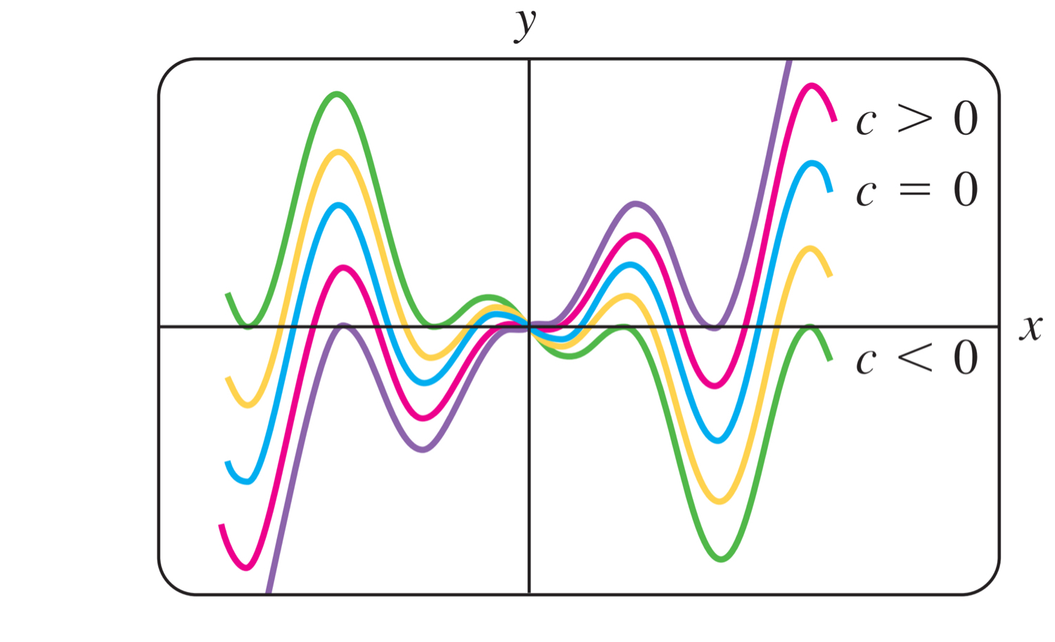
For example, the one-parameter family of solutions given by \(y=cx-x \cos x\) is an explicit solution of the linear first-order differential equation \(xy'-y= x^2 \sin x\) (Verify this). Figure 1 below taken from Zill and Cullen, shows the graphs of some of the solutions in this family governed by infinite values of the arbitrary constant \(c\). The solution \(y=-x \cos x\), the blue curve in the figure, is a particular solution corresponding to the value of the arbitrary constant \(c=0\).

Figure 1: A one-parameter family of solutions

Exercise:

Draw a rough sketch or use a graphing calculator like Desmos to find the family of solution curves for the following differential equations:

1. \(y'=\cos x; \quad y=\sin x + c\)
2. \(y'=-0.2y, \quad y=Be^{-0.2t}\)

Did you get it?

Check your understanding of some of the concepts covered at this stage by attempting the DYGIT? on Solutions of ODEs. This is a formative assessment task and does not count for marks so please do it on your own to ascertain your own learning.

2.5 Methods of Solution for Ordinary Differential Equations

Euler’s Number and Ordinary Differential Equations

In the next section we shall familiarize ourselves with some interesting aspects of the behaviour of an important function and its derivatives that will appear in the solutions to differential equations that will follow thereafter.

Let us consider the function \(y = e^{x}\). This function has many interesting characteristics. For example, consider its derivative, \[\begin{equation*} \dfrac{d}{dx} e^{x} =\lim_{h \to 0}{\dfrac{e^{x + h} - e^{x}}{h}}. \end{equation*}\] If we simply factor out the \(e^{x}\) and note it is not affected by the limit, we get the following, \[\begin{equation*} \dfrac{d}{dx}e^{x} = e^{x} \lim_{h \to 0}{\dfrac{e^{h} - 1}{h}}. \end{equation*}\] With a simple substitution of \(n = e^{h}-1\) and some algebraic manipulation we can show that this is equivalent to \[\begin{equation} \dfrac{d}{dx} e^{x} = e^{x}\dfrac{1}{\lim_{n \to 0}\ln{(1+n)^{\dfrac{1}{n}}}}. \tag{2.7} \end{equation}\] At this point we note that \[\begin{equation} e = \lim_{n \to 0}{(1+n)^{\dfrac{1}{n}}}, \tag{2.8} \end{equation}\] where both of these have an approximate solution of 2.7182818284… We call \(e\) Euler’s number. Now substituting Equation (2.8) into Equation (2.7), we find a useful result. \[\begin{equation} \dfrac{d}{dx} e^{x} = e^{x}. \end{equation}\] Using this knowledge we can consider evaluating the derivative of \[\begin{equation} y = \ln{x}. \tag{2.9} \end{equation}\] After a simple manipulation of Equation (2.9), we get \[\begin{equation*} e^{y} = x. \end{equation*}\] Applying implicit differentiation to this we get \[\begin{equation*} e^{y} \dfrac{dy}{dx} = 1. \end{equation*}\] Rearranging we find \[\begin{equation*} \dfrac{dy}{dx} = \dfrac{1}{e^{y}}. \end{equation*}\] By substituting Equation (2.9) into this we get \[\begin{equation*} \dfrac{dy}{dx} = \dfrac{1}{e^{\ln{x}}}, \end{equation*}\] which simplifies to our next useful result. \[\begin{equation*} \dfrac{d}{dx} \ln{x} = \dfrac{1}{x}. \end{equation*}\] There is a special relationship between the instantaneous rate of change of a function and the function itself. This is a general pattern that we observe when studying rates of change. In addition, the number \(e\) shall play an important role in the solution to many models.

We will consider three particular methods of solution for ordinary differential equations in this course:

2.5.1 The Method of Direct Integration

2.5.2 The Method of Separation of Variables

2.5.3 The Method of Undetermined Coefficients

These are just three analytical methods for finding solutions to differential equations. There are numerous other analytical ndd numerical methods you will encounter in Mathematics, Physics, and further studies in Applied Mathematics.

Before delving in to the Methods section, I would like to draw your attention back to the preceding Chapter on the Prerequisites for this course. It would be worthwhile digging out your Calculus notes now. Here is a quick preamble:

You should also watch this recap of Section 2.3 before continuing as knowing how to correctly classify a differential equation is going to be essential when we decide which method of solution is appropriate for a given DE.

2.5.1 The Method of Direct Integration

The Method of Direct Integration can be used for \(n\)-th order differential equations, provided that they are differential equations that can be written in the standard form: \[\begin{equation} \dfrac{d^n y}{dx^n}=g(x). \tag{2.10} \end{equation}\]

Notice the following key classification criteria:

• The left hand side of the differential equation in (2.10) contains a single derivative of the dependent variable, of any order. The key here is that there are not multiple derivatives of the dependent variable.
• The derivative of the dependent variable is linear, meaning its degree is at most one, and there contains no products of the dependent variable with this derivative.
• The right hand side of the differential equation in (2.10) is a function of the independent variable only, i.e. \(g=g(x)\). This may include a constant/non-zero function of the independent variable. This means that the right hand side of the differential equation cannot contain any term or function involving the dependent variable.

If these classification criteria are met, the differential equation can be solved using the Method of Direct Integration. In this case, you can integrate the differential equation a sufficient number of times (\(n\) times in (2.10)) until \(y\) is found.

For example, the equation \[\begin{equation*} \dfrac{d^2 y}{dx^2}= x^3+3x+1, \end{equation*}\] satisfies the aforementioned criteria as the left hand side contains a single derivative of the dependent variable \(y\) that is linear and of the second order, while the right hand side contains some function of the independent variable \(x\). However, the equation \[\begin{equation} \dfrac{d x}{dt}= 3t+x^2, \end{equation}\] does not meet the criteria for the Method of Direct Integration. Even though the left hand side contains a single derivative of the dependent variable \(x\) that is linear and of the first order, the right hand side contains some function of the independent and dependent variable, i.e. \(g=g(t,x)\). What about the differential equation \[\begin{equation} y''+y'= x^3+3x+1, \end{equation}\] where \(y=y(x)\)? While the right hand side contains some function of the independent variable \(x\) only, the left hand side contains both a second and first derivative of the dependent variable, thus the Method of Direct Integration cannot be used here.

Remark. Please note here that a differential equation may not present itself in the form set out in Equation (2.10). Sometimes, manipulation will be required in order to write a given DE in this form before you can apply the method. But it is equally important that you do not force an equation to meet this form if it cannot be done. All that means is the differential equation cannot be solved using this method, and that another method may be applicable.

For example, do the following differential equations meet the criteria to use the Method of Direct Integration? \[\begin{equation} y''= x^3+3x-2y''+1, \end{equation}\] and \[\begin{equation} \left(\dfrac{d^2 y}{dx^2}\right)^{2}= x^3+3x+1. \end{equation}\]

Remark. It is important to remember the reasons why we were interested in classifying a differential equation. Hopefully you can see now how certain elements of classification are key markers to determine when a method of solution is applicable.

Once a given differential equation is shown to meet the form specified in Equation (2.10), the method of solution is simple: integrate both sides of the differential equation with respect to the independent variable \(x\), i.e. \[\begin{equation} \int \dfrac{d^n y}{dx^n} dx=\int g(x) dx. \end{equation}\] You then need to integrate this differential equation \(n\) times sequentially to get the following solution for the dependent variable \(y\):
\[\begin{equation} y=G(x_1)+G(x_2)+...+G(x_n)+c_1+c_2+...+c_n, \tag{2.11} \end{equation}\] where \(G(x_i)\) represents the antiderivatives, and \(c_i\) the constants of integration that result from integrating the differential equation \(n\) times. Equation (2.11) represents the general solution of the differential equation (2.10) by using the Method of Direct Integration.

Let us look at a simple first order case. This is what I mean:

Let us now consider some examples:

Examples

1. \(\dfrac{d y}{dx}+\sin 2x=0\)

2. \(\dfrac{d^3 y}{dx^3}=\sin 2x+e^{-2x}+x^2+x+7\)

Notice from the above example that:

• We had a third order derivative and we needed to integrate three times to find the solution for the dependent variable \(y\). In other words, the order of the differential equation dictates how many integration you need to do.
• These three integrations resulted in three arbitrary constants. In other words, the order of the differential equation will dictate the parameter of the family of solution curves.
• When integrating the differential equation the second and third time, it is imperative that you remember to integrate the terms containing any arbitrary constant as well.
• Be wary of your signs when integrating.

Did you get it?

Check your understanding of some of the concepts covered at this stage by attempting the DYGIT? on Direct Integration. This is a formative assessment task and does not count for marks so please do it on your own to ascertain your own learning.

2.5.2 The Method of Separation of Variables

Unlike the Method of Direct Integration outlined in 2.5.1, the Method of Separation of Variables can only be used for first-order differential equations.

Consider a first-order differential equation of the form \[\begin{equation} \dfrac{d y}{dx}=g(x)h(y). \tag{2.12} \end{equation}\]

Notice the following key classification criteria:

• The left hand side of the differential equation in (2.12) contains a single derivative of the dependent variable that is of the first order. The key here also is that there are not multiple derivatives of the dependent variable, only the first derivative.
• The first derivative of the dependent variable is linear, meaning its degree is at most one.
• The right hand side of the differential equation in (2.12) consists of the product of distinct functions of the dependent variable \(y\) and the independent variable \(x\), i.e. it contains a separate and distinct product of functions \(g=g(x)\) and \(h=h(y)\). Here also, the functions \(g\) and \(h\) may include a constant/non-zero function of the dependent or independent variable respectively. This means that the right hand side of the differential equation may contain terms or functions involving the dependent variable, provided it is a product with the terms or functions involving the independent variable.

If these classification criteria are met, the differential equation can be solved using the Method of Separation of Variables. For example, the equation \[\begin{equation*} \dfrac{d y}{dx}= y^2 x e^{3x+4y}, \end{equation*}\] is separable as it satisfies the aforementioned criteria as the left hand side contains a single first derivative of the dependent variable \(y\) that is linear and of the first order, while the right hand side contains a product of a function of the independent variable (\(g(x)=xe^{3x}\)), and a function of the dependent variable (\(h(y)=y^2e^{4y}\)). Notice that some manipulation was required here. However, the equation \[\begin{equation} \dfrac{d x}{dt}= x +\sin t, \end{equation}\] is not separable as it does not meet the criteria for the Method of Separation of Variables. Even though the left hand side contains a single derivative of the dependent variable \(x\) that is linear and of the first order, there is no way of expressing the right hand side \(x +\sin t\) as a product of a function of the independent variable \(t\) (\(g(t)\)), and a function of the dependent variable \(x\) (\(h(x)\)). Try your best :)

Remark. Please note again here that a differential equation may not present itself in the form set out in Equation (2.12). Sometimes, manipulation will be required in order to write a given DE in this form before you can apply the method. But it is equally important that you do not force an equation to meet this form if it cannot be done. All that means is the differential equation cannot be solved using this method, and that yet another method may be applicable.

Such a differential equation as written in the form given in Equation (2.12) is called separable since it is possible to separate the dependent and independent variables on different sides of the equation, i.e. \[\begin{equation*} \dfrac{1}{h(y)} \dfrac{d y}{dx}=g(x). \end{equation*}\] Under these specific circumstances when we have a first derivative only, we can treat the differentials/infinitesimals \(dy\) and \(dx\) as normal algebraic quantities and multiply or divide them on either side of the equation. This means that we can separate the dependent and independent variables on different sides of the equation along with its associated differential, i.e. \[\begin{equation*} \dfrac{1}{h(y)} dy=g(x) dx. \end{equation*}\] Once we have isolated the functions of the dependent variable \(y\) and its associated differential \(dy\), and the functions of the independent variable \(x\) and its associated differential \(dx\) on either side of the equation, we can then integrate both sides of the equation with respect to its associated differential, i.e. \[\begin{equation*} \int \dfrac{1}{h(y)} dy=\int g(x) dx. \end{equation*}\] We can then use the rules of integration as well as some algebraic manipulation in order to find a solution for the dependent variable \(y\). Hence, the general solution of Equation (2.12) is given by \[\begin{equation*} \int \dfrac{1}{h(y)} dy=\int g(x) dx +c, \end{equation*}\] where \(c\) is the constant of integration. Note here that even though we are computing an integral on either side of the equation, we only require one constant of integration due to the nature of arbitrary constants.

Remark. It is important to note here that a separable ordinary differential equation may not necessarily be analytically solvable as the resulting integrals may not always be reducible to elementary functions.

Even when this integration is analytically possible, it is oftentimes the case that this solution for the dependent variable \(y\) will be in implicit form. We will endeavour as much as possible to write this solution in explicit form as outlined in Definition 2.11. Again, do not force a solution into explicit form if it cannot be written as such. We will leave such solutions in implicit form. If a question does not state otherwise, you can assume that I require an explicit solution. When an implicit solution is deemed sufficient, I will state that “you may leave your solution in implicit form”.

Examples

1. \(\dfrac{d y}{dx}=2\)

2.  \(\dfrac{d y}{dx}=\sin x\)

3.  \(\dfrac{d y}{dx}=xy\)

4.  \(\dfrac{d y}{dx}-2y=0\)

Try this on your own

5.  \(\dfrac{d y}{dx}-2y=3\)

(Ignore the reference in the beginning to page numbers and notes. This is my video from last year.)

6.  \(\dfrac{d y}{dx}-\dfrac{y}{x}=0\)

Try this on your own

7.  \(\dfrac{d y}{dx}-2y^2+5y=3\)

This example requires a full understanding of the algebraic technique called partial fraction decomposition which you have covered in Mathematics.

Thinking Questions:

1. Can a given differential equation meet the criteria to be solved by using either the Method of Direct Integration, or the Method of Separation of Variables?
2. If so, what does that tell you?
3. If so, can you think of examples of such differential equations?
4. If so, go back to all the examples of differential equations you have seen thus far, and observe them through this dual lens.

Exercise

In the problems below, solve the given differential equation for its general solution in explicit form by using either the method of direct integration, separation of variables, or both.

1. \(\dfrac{d^2 x}{dt^2}+16x=0\)

2. \(\dot x+5x=10\)

3. \(\dfrac{d^3 y}{dx^3}-2y=0\)

4. \(y\dfrac{d y}{dx}=\sin 5x\)

5. \(\dfrac{d^3 y}{dx^3}=\sin 5x\)

6. \((1+x) dy-y dx=0\), where \(y=y(x)\)

7. \(\dfrac{d y}{dx}=(x+1)^2\)

8. \(dx+e^{3x}dy=0\), where \(y=y(x)\)

9. \(\dfrac{d^3 y}{dx^3}-2y^2=0\)

10. \(\dfrac{d^3 y}{dx^3}-2x^2=0\)

11. \(\dfrac{d S}{dt}-\dfrac{5S}{t}=0\)

12. \(y\dfrac{d y}{dx}=3y^2+1\)

13. \(y'-3y^2-y=0\)

14. \(\dfrac{d x}{dt}-x^2=-4\)

15. \(t \dot x -(1+t)x=0\)

16. \((a^2-x^2)y'+xy=0\), where \(a\) is a constant

17. \(\dfrac{d y}{dx}-\dfrac{y+3}{x^2-3x+2}=0\)

18. Find an implicit general solution to the following equation \(\dfrac{y}{x^2}\dfrac{d y}{dx}+e^{2x^{3}+y^{2}}=0\)

Did you get it?

Check your understanding of some of the concepts covered at this stage by attempting the DYGIT? on Separation of Variables. This is a formative assessment task and does not count for marks so please do it on your own to ascertain your own learning.

2.5.3 The Method of Undetermined Coefficients

Recall that the solution to a differential equation is a function, expressed in the common set of variables that satisfies the original equation. More generally, differential equations can involve collections of equations which relate collections of functions. A solution to such a collection of equations is necessarily a function that satisfies all the relations of the original equation for some collection of the common variable set. This means that a differential equation is well-defined only for some collection of parameters that specify the differential equation. Our task has been to find these solutions and understand the limitations of these solutions when moving from point to point in the space of parameters that specify the original differential equation for some initial data.

Let us begin this section by revising the definition of homogeneity for a linear ordinary differential equation:

Definition 2.16 (Homogeneity of a Linear Ordinary Differential Equation) A linear nth-order differential equation of the form \[\begin{equation} a_{n}(x)\dfrac{d^n y}{dx^n}+a_{n-1}(x)\dfrac{d^{n-1} y}{dx^{n-1}}+\dots+ a_{2}(x)\dfrac{d^2 y}{dx^2}+a_{1}(x)\dfrac{d y}{dx}+a_{0}(x)y=0 \tag{2.13} \end{equation}\] is said to be homogeneous, whereas an equation \[\begin{equation} a_{n}(x)\dfrac{d^n y}{dx^n}+a_{n-1}(x)\dfrac{d^{n-1} y}{dx^{n-1}}+\dots+ a_{2}(x)\dfrac{d^2 y}{dx^2}+a_{1}(x)\dfrac{d y}{dx}+a_{0}(x)y=g(x) \tag{2.14} \end{equation}\] with \(g(x)\) not identically zero, is said to be non-homogeneous.

For example, \(2y''+3y'-5y=0\) is a homogeneous linear second-order differential equation, whereas \(x^3 y'''+6y'+10y=e^x\) is a non-homogeneous linear third-order differential equation.

We shall see that to solve a non-homogeneous linear equation as in Equation (2.14), we must first be able to solve the associated homogeneous equation in Equation (2.13).

The general or complete solution of (2.13) must contain \(n\) arbitrary constants since solving it implicitly requires \(n\) integrations. If the value of the function and its derivatives are known at sufficiently many points then it is possible to compute the values of these constants. If these values are all known at \(x = x_{0}\), for some \(x_{0}\), they are called initial conditions and the problem of solving the DE is called an initial value problem (IVP), otherwise it is called a boundary value problem (BVP).

A particular solution to a given differential equation is found by determining the general solution to the equation up to some collection of constants, which are determined using some data. This data specifies the function values at some set of parameter values. A minimal set of data must supply sufficient information to specify the function value at each point in parameter space. This means that the value of the function and any number of its derivatives must be entirely specified at each parameter value where the equation is well-defined. This data can be specified in one of two ways which leads to two kinds of problems.

Definition 2.17 (Initial Value Problem) Supply one data point to the function itself and one data point for each derivative of the function. This is natural for problems where an initial displacement, initial velocity and so on, are specified. A problem of this kind is called an initial value problem (IVP).

Definition 2.18 (Boundary Value Problem) Supply multiple data points for some subset of derivatives of the function. This occurs when the function data is defined within some bounded region and the data is provided at the boundary of the region. A problem of this kind is called a boundary value problem (BVP).

For now, we shall focus on IVP’s.

We will now turn our attention to second-order linear non-homogeneous ordinary differential equations with constant coefficients with the standard form \[\begin{equation} a y'' + b y' + c y = g(x), \tag{2.15} \end{equation}\] where \(y=y(x)\), and \(a\), \(b\), and \(c\) are constants, \(a \neq 0\); and \(g(x) \neq 0\).

It has a corresponding homogeneous equation \[\begin{equation} a y'' + b y' + c y = 0. \tag{2.16} \end{equation}\]

Definition 2.19 (Complementary Function of a Linear Ordinary Differential Equation) The general solution to the homogeneous equation (2.16) is called the complementary function of the non-homogeneous equation, and is denoted by \(y_{c}\).

Definition 2.20 (Particular Integral of a Linear Ordinary Differential Equation) A solution to the non-homogeneous equation (2.15) is called the particular integral of the same equation, and is is denoted by \(y_{p}\).

The general solution of Equation (2.13) \(y_c\) is called the complementary function for Equation (2.14). In other words, to solve a non-homogeneous linear differential equation, we first solve the associated homogeneous equation and then find any particular solution of the non-homogeneous equation. Any function \(y_p\), free of arbitrary constants, that satisfies Equation (2.14) is said to be a particular integral of the equation.

Definition 2.21 (General Solution of a Linear Ordinary Differential Equation) The general solution of the nth-order non-homogeneous linear equation (2.14) can be expressed in the form \[\begin{equation} y=\text{complementary function} + \text{any particular integral}=y_{c}+y_{p}, \end{equation}\] where \(y_{p}\) is any specific function that satisfies the non-homogeneous equation, and \(y_{c}\) is a general solution of the corresponding homogeneous equation (2.13).

The term \(y_{c}\) contains \(n\) arbitrary constants. If the values of \(y\) in (2.13) and its derivatives are known at sufficiently many points, then these \(n\) arbitrary constants may be computed using the general solution.

Remark. It should be noted that the complementary function is never actually a solution of the given non-homogeneous equation. It is merely taken from the corresponding homogeneous equation as a component that, when coupled with a particular integral, gives us the general solution of a non-homogeneous linear equation. On the other hand, the particular integral is necessarily always a solution of the said non-homogeneous equation.

2.5.3.1 Homogeneous Linear Equations with Constant Coefficients

Let us first consider a first-order, linear, homogeneous differential equation with constant coefficients.

Consider the equation \[\begin{equation} \dfrac{d y}{dx} - a y = 0, \end{equation}\] where \(a\) is a constant and is independent of \(x\). This is a first order, linear, homogeneous DE with constant coefficients. Notice that this equation states that the derivative of the dependent variable is proportional to the dependent variable itself. We may integrate directly as follows. \[\begin{align*} \dfrac{d y}{dx} - ay &= 0, \\ \dfrac{d y}{dx} &= ay, \\ \int{d y \dfrac{1}{y}} &= \int{a d x} \\ \ln{y} &= ax + c_{1} \\ \implies y &= c_{2} e^{ax}. \end{align*}\] The parameter appearing in the original differential equation appears as a parameter in the solution. Note the appearance of the exponential term \(e^{ax}\) in the solution. This is a common pattern that arises in solutions to linear differential equations with terms proportional to the dependent variable and derivatives thereof. This follows from the identity \[\begin{equation} \dfrac{d}{dx} e^{a x} = a e^{a x}. \end{equation}\] We shall use this to construct solutions to linear differential equations with constant coefficients.

Let us consider a few examples:

Now, let us extend this for the case of a second-order, linear, homogeneous differential equation with constant coefficients as given in Equation (2.16):

\[\begin{equation} a y'' + b y' + c y = 0, \end{equation}\] where \(y=y(x)\), and \(a\), \(b\), and \(c\) are independent of \(y\) and \(x\).

Since the right-hand side of (2.16) is zero, \(y\) is a function that is not greatly changed by differentiation. It actually portrays the character of the exponential function. To solve this equation, select a suitable trial solution of the form \(y_{c}(x) = Ae^{\lambda x}\), where \(A\) is an arbitrary constant, and \(\lambda\) is a yet to be determined constant. Direct substitution of the trial solution into (2.16) yields an algebraic equation \[\begin{equation} a \lambda^{2} + b \lambda + c = 0 \tag{2.17} \end{equation}\] We call (2.17) the characteristic equation or auxiliary equation of the homogeneous equation (2.16).

The roots of (2.17) are \[\begin{equation*} \lambda_{1} = \dfrac{-b - \sqrt{b^{2} - 4 a c}}{2a} \quad \text{and} \quad \lambda_{2} = \dfrac{-b + \sqrt{b^{2} - 4 a c}}{2a}. \end{equation*}\] The nature of the solutions of (2.17) depend on the values \(\lambda_{1}\) and \(\lambda_{2}\) and we shall examine each separately. In each case, consider the behaviour of the discriminant of (2.17), for the cases that \(b^{2} - 4 a c\) is positive, negative or zero.

We will require the following definition before we observe the nature of the solutions of (2.17).

Definition 2.22 (Superposition Principle) Consider Equation (2.13) with \(g(x) = 0\), giving \[\begin{equation} c_{n} \dfrac{d^{n}y}{dx^{n}} + c_{n-1} \dfrac{d^{n-1}y}{dx^{n-1}} + \cdots + c_{1} \dfrac{d y}{dx} + c_{0} y = 0. \end{equation}\] Suppose \(y_{1}, y_{2}, y_{3}, \dots, y_{n}\) are solutions of this \(n\)-th order linear, homogeneous DE, then \[\begin{equation*} y = \sum_{i = 1}^{n}{c_{i} y_{i} } \end{equation*}\] where \(c_{i}\) are arbitrary constants, is also a solution. This is called the superposition principle.

In the discussion to follow, we shall also make extensive use of the following definition.

Definition 2.23 (Linearly Dependent and Independent Functions) Consider two functions \(f(x)\) and \(g(x)\) and let \(a\) and \(b\) be constants, independent of \(x\). If the equation \[\begin{equation*} a f(x) + b g(x) = 0, \end{equation*}\] has solutions \(a \neq 0\) and \(b \neq 0\) then \(f(x)\) is some constant multiple of \(g(x)\). In such cases, \(f(x)\) and \(g(x)\) are linearly dependent. If there exists no solutions \(a \neq 0\) and \(b \neq 0\) then \(f(x)\) and \(g(x)\) are linearly independent functions.

Consider the following cases:

Case 1: Distinct real roots \(b^{2} - 4 a c > 0\)

Here, \(\lambda_{1}\) and \(\lambda_{2}\) are real and distinct and (2.17) has two distinct solutions, \[\begin{equation*} y_{1}(x) = e^{\lambda_{1} x} \quad \text{and} \quad y_{2}(x) = e^{\lambda_{2} x}. \end{equation*}\] Since (2.16) is second order it must contain two arbitrary constants. These two solutions are linearly independent. Additionally, (2.17) is linear and homogeneous, so by the superposition principle, any linear combination of two solutions is also a solution. Hence, the general solution to (2.16) is \[\begin{equation*} y(x) = c_{1} e^{\lambda_{1} x} + c_{2} e^{\lambda_{2} x}, \end{equation*}\] with \(c_{1}\) and \(c_{2}\) as arbitrary constants.

Example

Consider the following equation, \[\begin{equation*} \ddot{x} + 3 \dot{x} + 2 x = 0, \end{equation*}\] and the initial data \(x(0) = 0\) and \(\dot{x}(0) = 1\). Let the trial solution take the form \(x(t) = A e^{\lambda t}\), then direct substitution of the trial solution into the given DE yields the auxiliary equation \[\begin{equation*} \lambda^{2} + 3 \lambda + 2 = 0. \end{equation*}\] with roots \(\lambda_{1} = -1\) and \(\lambda_{2} = -2\). Hence, the general solution is \[\begin{equation*} x(t) = c_{1} e^{-t} + c_{2} e^{-2t}, \end{equation*}\] where \(c_{1}\) and \(c_{2}\) are arbitrary constants. We get a particular solution to this equation by evaluating the general solution at the given initial data points and solving for the constants \(c_{1}\) and \(c_{2}\). The first initial condition \(x(0) = 0\) implies that \(c_{1} = -c_{2}\), and the second initial condition \(\dot{x}(0) = 1\) implies that \(1 = -c_{1} - 2 c_{2}\). When combined, these two relations yield \(c_{1} = 1\) and \(c_{2} = -1\). Therefore, a particular solution is \[\begin{equation*} x(t) = e^{-t} - e^{-2t}. \end{equation*}\]

Case 2: Repeated real roots \(b^{2} - 4 a c = 0\)

The roots of (2.17) coincide and \(\lambda_{1} = \lambda_{2} = \lambda = -\dfrac{b}{2a}\), so there exists a solution \[\begin{equation*} y_{1}(x) = e^{\lambda x}. \end{equation*}\] Since the DE in question is second order, and must contain two arbitrary constants, we conclude that there must exist a second solution \(y_{2}\). To determine this second solution, consider a second trial solution \(y = xe^{\lambda x}\), which is similar to, but linearly independent, of the first trial solution. Direct substitution of this trial solution into (2.16) yields \[\begin{equation*} (2a \lambda + b) e^{\lambda x} + (a \lambda^{2} + b \lambda + c) x e^{\lambda x} = 0. \end{equation*}\] Since \(e^{\lambda x}\) and \(xe^{\lambda x}\) are linearly independent, we require that the coefficients \((2a \lambda + b)\) and \((a \lambda^{2} + b \lambda + c)\) are simultaneously equal to zero for all values of \(t\). Solving this set of simultaneous equations yields again \(\lambda = - \dfrac{b}{2a}\). The second solution is \[\begin{equation*} y_{2}(x) = x e^{\lambda x}. \end{equation*}\] Combine \(y_{1}\) and \(y_{2}\) using the superposition principle to form the general solution, \[\begin{equation*} y(x) = c_{1} e^{\lambda x} + c_{2} x e^{\lambda x}, \end{equation*}\] with \(c_{1}\) and \(c_{2}\) as arbitrary constants.

Errata: Please note that in the video below, the example should be \(y''-2y'+y=0\).

Example

Consider the following equation, \[\begin{equation*} \ddot{x} - 4 \dot{x} + 4 x = 0, \end{equation*}\] and take \(x(t) = A e^{\lambda t}\) as the trial solution. The associated auxiliary equation is \[\begin{equation*} \lambda^{2} - 4 \lambda + 4 = 0, \end{equation*}\] with a double root \(\lambda = 2\), or we say that \(\lambda = 2\) with multiplicity two. Therefore, one solution to this DE is \[\begin{equation*} x_{1}(t) = e^{2t}. \end{equation*}\]

Note:

• Clearly, this is not the complete solution as the number of arbitrary constants is not equal to the order of the DE. There are several ways to solve for another function which also satisfies the given equation. In order to choose another function, we use our original solution multiplied by a single degree of the independent variable, in this case \(t\), and replace the original constant with a different one.

Thus, a second solution to this DE is \[\begin{equation*} x_{2}(t) = t e^{2t}. \end{equation*}\] Combining \(x_{1}\) and \(x_{2}\) yields the general solution \[\begin{equation*} x(t) = c_{1} e^{2t} + c_{2} t e^{2t}. \end{equation*}\]

The appearance of a second solution, which is equal to the product of some function of the independent variable and the first solution, is a common feature of DEs with zero discriminant.

Case 3: Complex conjugate roots \(b^{2} - 4 a c < 0\)

Here, \(\lambda_{1}\) and \(\lambda_{2}\) are complex conjugate roots of the auxiliary equation (2.17). Hence, (2.16) has two distinct solutions, \[\begin{equation*} y_{1}(x) = e^{\lambda_{1} x} \quad \text{and} \quad y_{2}(x) = e^{\lambda_{2} x}. \end{equation*}\] Again, since (2.16) is second order, it must contain two arbitrary constants. Also, by the linearity and homogeneity of (2.16), the superposition principle implies that any linear combination of these two solutions is a solution. Hence, the general solution to (2.16) is \[\begin{equation*} y(x) = c_{1} e^{\lambda_{1} x} + c_{2} e^{\lambda_{2} x}, \end{equation*}\] with \(c_{1}\) and \(c_{2}\) as complex constants. Typically, (2.16) is specified with real coefficients and the requirement that \(y(x)\) is a real-valued function. Since \(\lambda_{1}\) and \(\lambda_{2}\) are complex conjugates, \(e^{\lambda_{1} x}\) and \(e^{\lambda_{2} x}\) are also complex conjugates. If \(y(x)\) is to be real-valued, then \(c_{1}\) and \(c_{2}\) must be complex conjugates.

We would like to rewrite these solutions in a more natural way, free of the complex numbers associated with the negative discriminant. To do this, define, \[\begin{equation*} \alpha = -\dfrac{b}{2a} \quad \text{and} \quad \beta = \dfrac{\sqrt{4 a c - b^{2}}}{2a}. \end{equation*}\] Rewrite the conjugate root pair as \(\lambda_{1} = \alpha - i \beta\) and \(\lambda_{2} = \alpha + i \beta\), where \(i \equiv \sqrt{-1}\). We can now rewrite \(y_{1}\) as, \[\begin{equation*} y_{1}(x) = e^{\lambda_{1} x} = e^{(\alpha - i \beta) x} = e^{\alpha x} e^{- i \beta x}. \end{equation*}\] Similarly, rewrite \(y_{2}\) as, \[\begin{equation*} y_{2}(x) = e^{\alpha x} e^{i \beta x}. \end{equation*}\] Recall the Euler identity, \[\begin{equation} e^{i \theta} = \cos{\theta} + i \sin{\theta}. \tag{2.18} \end{equation}\] Rewriting the general solution using (2.18) yields, \[\begin{align*} y(x) &= c_{1} e^{\alpha x} e^{-i \beta x} + c_{2} e^{\alpha x} e^{i \beta x} \\ &= c_{1} e^{\alpha x} \left( \cos{\beta x} - i \sin{\beta x} \right) + c_{2} e^{\alpha x} \left( \cos{\beta x} + i \sin{\beta x} \right) \\ &= e^{\alpha x} \left( \cos{\beta x} (c_{1} + c_{2}) + i \sin{\beta x} (c_{2} - c_{1}) \right). \end{align*}\] Define, \(c_{3} = c_{1} + c_{2}\) and \(c_{4} = i(c_{2} - c_{1})\), then \[\begin{equation} y(x) = e^{\alpha x} \left( c_{3} \cos{\beta x} + c_{4} \sin{\beta x} \right), \end{equation}\] where \(c_{3}\) and \(c_{4}\) are to be determined constants. Note that if \(c_{1}\) and \(c_{2}\) are complex conjugates, then \(c_{3}\) and \(c_{4}\) are real-valued.

Remark. We always write our solution in its real form.

Example

Consider the following equation, \[\begin{equation*} \ddot{x} + 4 \dot{x} + 5 x = 0, \end{equation*}\] and let the trial solution take the form \(x(t) = Ae^{\lambda t}\). Then direct substitution of the trial solution into the given DE yields the auxiliary equation \[\begin{equation*} \lambda^{2} + 4 \lambda + 5 = 0. \end{equation*}\] with roots \(\lambda_{1} = -2 - i\) and \(\lambda_{2} = -2 + i\). Here, \(\alpha=-2\) and \(\beta=1\). Hence, the general solution is \[\begin{equation*} x(t) = e^{-2t} \left( c_{1} \cos{t} + c_{2} \sin{t} \right), \end{equation*}\] with \(c_{1}\) and \(c_{2}\) as arbitrary constants.

Notice that the general solution is now a product of an exponential term and a pair of trigonometric functions. This is a common feature of homogeneous DEs with a negative discriminant.

Additional Examples

1. \(y''+4y'+7y=0\)

2. \(\dfrac{d^2 y}{dx^2}+4\dfrac{d y}{dx}+4y=0\)

3. \(\dfrac{d^2 x}{dt^2}-4x=0\)

Exercise

1. Find the general solution to the following differential equations, and hence verify your solution.

   1. \(\dfrac{d^2 x}{dt^2}+16x=0\) (This should look familiar)

   2. \(\dfrac{d^2 y}{dx^2}-\dfrac{d y}{dx}-2y=0\)

   3. \(\dfrac{d^2 x}{dt^2}+4\dfrac{d x}{dt}=0\)

   4. \(\dfrac{d^2 S}{dt^2}-2\dfrac{d S}{dt}+S=0\)

   5. \(\dfrac{d^2 S}{dt^2}-2\dfrac{d S}{dt}+5S=0\)

2. Find the solution to the DE \(\ddot{x} + 2 \dot{x} -3 x = 0\), given that \(x(0) = 0\) and \(\dot{x}(0) = 1\).

3. Given the DE \(\ddot{x} - 4 \dot{x} + 4 x = 0\).

   1. Find the general solution.
   2. Show that the initial conditions \(x(0) = 1\) and \(\dot{x}(0) = 0\) give the particular solution \(x(t)=(1-2t) e^{2t}\).
   3. Determine the initial conditions which gives the particular solution \(x(t)=te^{2t}\).

Did you get it?

Check your understanding of some of the concepts covered at this stage by attempting the DYGIT? on The Method of Undetermined Coefficients: Homogeneous Linear Equations with Constant Coefficients. This is a formative assessment task and does not count for marks so please do it on your own to ascertain your own learning.

Next, we will look at how to find the particular integral of a given non-homogeneous differential equation with constant coefficients.

2.5.3.2 Undetermined Coefficients: Superposition Approach

To solve a non-homogeneous linear differential equation as in (2.14) for its general solution \(y\), we have to do two things: to find the complementary function \(y_c\) which is the general solution of the associated homogeneous DE (2.13), and to find any particular solution \(y_p\) of the non-homogeneous equation (2.14) which we refer to as the particular integral.

In this section, we are interested in now finding a solution of the non-homogeneous linear equation by focusing on finding the particular integral \(y_{p}\).

The Method of Undetermined Coefficients (sometimes referred to as the method of Judicious Guessing) is a systematic way of using an “educated or reasonable guess” to determine the general form/type of the particular integral \(y_{p}\) based on the non-homogeneous term \(g(x)\) in the given non-homogeneous equation (2.14). We often refer to this guess as the ansatz. If the initial guess for the ansatz leads to contradictions or does not yield the expected number of arbitrary constants, it means your initial ansatz was not chosen correctly and an improved and adjusted guess is required. This process is repeated until the most general solution has been obtained.

The underlying feature of this method is a conjecture about the form of \(y_p\) that is motivated by the kinds of functions that make up the input function \(g(x)\).

The basic idea is that many of the most familiar and commonly encountered functions have derivatives that vary little (in the form/type of function) from their parent functions: exponential, polynomials, sine and cosine. Consequently, when those functions appear in \(g(x)\), we can predict the type of function that the solution \(y_{p}\) would be.

This general method is limited to linear DEs such as (2.14) where the coefficients \(a_i\), \(i=0, 1, . . . , n\) are constants. As well as this, the functions that constitute \(g(x)\) must be either be

• a constant \(k\),
• a polynomial function,
• an exponential function \(e^{ax}\) where \(a\) is a number,
• a sine or cosine function \(\sin bx\) or \(\cos bx\) where \(b\) is a number, or
• finite sums and products of these functions.

The set of functions that consists of constants, polynomials, exponentials of the form \(e^{ax}\), and sines and cosines has the remarkable property that derivatives of their sums and products are again sums and products of constants, polynomials, exponentials \(e^{ax}\), and sines and cosines. Because the linear combination of derivatives must be identical to \(g(x)\), it seems reasonable to assume that \(y_p\) has the same form as \(g(x)\).

To implement this method, we follow these steps:

1. Check if the given ordinary differential equation is linear with constant coefficients.
2. Check if the function \(g(x)\) satisfies the aforementioned criteria.
3. Write down the (best guess) form of the ansatz \(y_{p}\), leaving the coefficient(s) undetermined. A surefire way to check that you chose the correct ansatz is by differentiating the given function \(g(x)\) at least twice, and then comparing \(g(x)\) and any of its computed derivatives with your chosen ansatz. If your ansatz most generally encapsulates the terms that appear in \(g(x)\) and any of its derivatives, then your chosen ansatz is most likely correct.
4. Compare your ansatz with the already found complementary function \(y_c\) for any duplication. If there is no duplication, we say that this ansatz is linearly independent from the complementary function. If there is any duplication, it means that the chosen ansatz and the complementary function are linearly dependent, and so we must adjust this initial ansatz until there is no longer any duplication. This is a crucial, and often misunderstood and overlooked step.
5. Compute \(y'_{p}\) and \(y''_{p}\) using the usual rules and techniques of differentiation, and then substitute these into the original differential equation.
6. Hence solve for the unknown coefficient(s) by matching to find the particular integral.

Remark. If you perform steps 3 and 4 correctly, you are guaranteed to choose the most general ansatz that is void of duplication.

This brings us to the following important Theorem:

Theorem 2.1 (Duplication between the ansatz and complementary function) The following theorem outlines the cases with and without duplication:

• If there is no duplication between your chosen ansatz for \(y_p\) and the complementary function \(y_c\), the form of the ansatz \(y_p\) is a linear combination of all linearly independent functions that are generated by repeated differentiations of g(x).

• If any choice for an ansatz \(y_p\) contains terms that duplicate terms in \(y_c\),then that \(y_p\) must be multiplied by \(x^n\), where \(x\) represents the independent variable, and \(n\) is the smallest positive integer that eliminates that duplication.

Note:

• We do not make any changes or adjustments to the complementary function \(y_c\). The only aspect we are allowed to adjust is our ansatz for the particular integral \(y_p\).

In the Table below, we illustrate some specific examples of \(g(x)\) in (2.14) along with the corresponding form of the trial ansatz for finding the particular integral. We are of course at this stage making an assumption that no function in the ansatz for the particular integral \(y_p\) is duplicated by a function in the complementary function \(y_c\).

\(g(x)\)	\(y_p\)
\(5\)	\(A\)
\(5x+7\)	\(Ax+B\)
\(-3x\)	\(Ax+B\) (Not \(Ax\) and not \(-Ax\))
\(5x^2-7x+9\)	\(Ax^2+Bx+C\)
\(5x^2-9\)	\(Ax^2+Bx+C\) (Not \(Ax^2+B\) and not \(Ax^2-B\))
\(x^3-x-1\)	\(Ax^3+Bx^2+Cx+D\) (Not \(Ax^3+Bx+C\) and not \(Ax^3-Bx-C\))
\(e^{5x}\)	\(Ae^{5x}\) (Note that \(e^{5x}\) is explicit in the guess)
\(\sin 4x\)	\(A \sin 4x +B \cos 4x\) (Not \(A\sin 4x\) and not \(A \sin x\))
\(\cos \sqrt{2}x\)	\(A\cos \sqrt{2}x+B\sin \sqrt{2}x\)
\(3x+e^{2x}\)	\(Ax+B+Ce^{2x}\) (Not \(Ax+Be^{2x}\))
\((9x-2)e^{5x}\)	\((Ax+B)e^{5x}\) (Not \((Ax+B)Ce^{5x}\)) Why?
\(e^{3x} \sin 5x\)	\(Ae^{3x} \sin 5x+Be^{3x} \cos 5x\) (Not \(Ae^{3x}(B\sin 5x+C\cos 5x)\))
\(xe^{3x}\cos x\)	\((Ax+B)e^{3x}\sin x+(Cx+D)e^{3x}\cos x\) (Understand this)

Worked Out Examples

We begin by first considering a few illustrative examples where the non-homogeneous term contains exponential functions of the form \(e^{ax}\).

1. An exponential function \(e^{ax}\) without duplication

Consider the DE \[\begin{equation*} \ddot{x} + 3 \dot{x} + 2x = e^{2t}. \end{equation*}\] The homogeneous part of this equation is \[\begin{equation*} \ddot{x} + 3 \dot{x} + 2x = 0. \end{equation*}\] Choosing \(x(t) = Ae^{\lambda t}\) as a trial solution yields the corresponding auxiliary equation, \[\begin{equation*} \lambda^{2} + 3 \lambda + 2 = 0, \end{equation*}\] which has roots \(\lambda_{1} = -1\) and \(\lambda_{2} = -2\). From these roots we construct the complementary function \[\begin{equation*} x_{c}(t) = c_{1} e^{-t} + c_{2} e^{-2t}. \end{equation*}\]

To construct the particular integral:

1. We note that the given DE is linear and has constant coefficients.

2. \(g(t)=e^{2t}\) satisfies the criteria and so the method is applicable.

3. We then can choose the ansatz to be \(x_{p}=A e^{2t}\).

4. We compare this ansatz to \(x_{c} = c_{1} e^{-t} + c_{2} e^{-2t}\) and notice that there is no duplication as the chosen ansatz is linearly independent of each term in the complementary function. Therefore, no adjustment is necessary.

5. We compute using chain rule \(x'_{p}=2A e^{2t}\) and \(x''_{p}=4A e^{2t}\), and substitute into the original equation to get \[\begin{align*} 4A e^{2t} + 6A e^{2t} + 2A e^{2t} &= e^{2t}, \\ 12A e^{2t} &= e^{2t}. \end{align*}\]

6. We can the solve for the undetermined coefficients by matching. And so for the above equation to hold, we can match coefficients, and so, \[\begin{equation*} 12 A = 1, \end{equation*}\] meaning that \(A = \frac{1}{12}\). This gives the particular integral \[\begin{equation*} x_{p}(t) = \frac{1}{12} e^{2t}. \end{equation*}\] Hence, the general solution is \[\begin{equation*} x(t) = x_{c}+x_{p} = c_{1} e^{-t} + c_{2} e^{-2t} + \frac{1}{12} e^{2t}. \end{equation*}\]

In order to find the values of \(c_{1}\) and \(c_{2}\), we would require two initial conditions.

2. An exponential function \(e^{ax}\) with duplication

Consider the DE \[\begin{equation*} \ddot{x} + 3 \dot{x} + 2x = e^{-t}. \end{equation*}\] The complementary solution to this DE is the same as in Example 1 above, i.e. \[\begin{equation*} x_{c}(t) = c_{1} e^{-t} + c_{2} e^{-2t}. \end{equation*}\]

To construct the particular integral:

1. We note that the given DE is linear and has constant coefficients.
2. \(g(t)=e^{-t}\) satisfies the criteria and so the method is applicable.
3. We then can choose the ansatz to be \(x_{p}=A e^{-t}\).
4. We compare this ansatz to \(x_{c} = c_{1} e^{-t} + c_{2} e^{-2t}\) and notice that there is duplication as the chosen ansatz is linearly dependent on the term \(c_{1} e^{-t}\) in the complementary function. What we mean is that and \(A e^{-t}\) and \(c_{1} e^{-t}\) are the same as \(A\) and \(c_1\) are just arbitrary constants. In other words, our chosen ansatz is a particular case of the complementary function, specifically when \(c_{1} = 1\), \(c_{2} = 0\) and \(A=1\). Therefore, an adjustment of our initial ansatz for the particular integral is necessary. We then adjust our guess using Theorem 2.1 so that there is no longer any duplication. We do this by multiplying the duplicated term in the ansatz \(x_p\) by one degree of the independent variable (in this case \(t\)). And so the adjusted ansatz is \(x_{p}(t) = A t e^{-t}\), which is similar to, but is now linearly independent of the particular cases of the complementary function.

Note:

• If this adjusted ansatz was still linearly dependent on any of the terms in the complementary function, we would carry on multiplying by another degree of the independent variable as per Theorem 2.1, and would only stop when there is no longer a duplication and the adjusted ansatz is linearly independent of the complementary function.

5. We compute using product and chain rule \(x'_{p}=A e^{-t}-At e^{-t}\) and \(x''_{p}=-2A e^{-t}+At e^{-t}\), and substitute into the original equation to get \[\begin{align*} -2A e^{-t} + At e^{-t} + 3(A e^{-t} - At e^{-t}) + 2At e^{-t} &= e^{-t}, \\ A e^{-t} &= e^{-t}. \end{align*}\]

6. We can the solve for the undetermined coefficients by matching. And so for the above equation to hold, we can match coefficients, and so, \[\begin{equation*} A = 1. \end{equation*}\] This gives the particular integral \[\begin{equation*} x_{p}(t) = t e^{-t}. \end{equation*}\] The general solution is then \[\begin{equation*} x(t) = x_{c}+x_{p} = c_{1} e^{-t} + c_{2} e^{-2t} + t e^{-t}. \end{equation*}\]

Remark. In general, if the right-hand-side of a non-homogeneous DE is a particular case of the complementary function, then the ansatz for the particular integral will need adjusting to account for this duplication.

It is common that non-homogeneous linear differential equations may have a non-homogeneous term of polynomial type. We would like to gain insight into the appropriate choice of trial solution for the particular integral in such cases.

3. A polynomial function

Consider the DE \[\begin{equation*} \ddot{x} + 3 \dot{x} + 2x = t^{2}. \end{equation*}\] The complementary solution to this DE is the same as in Examples 1 and 2, which is \[\begin{equation*} x_{c}(t) = c_{1} e^{-t} + c_{2} e^{-2t}. \end{equation*}\]

To construct the particular integral:

1. We note that the given DE is linear and has constant coefficients.
2. We note that the non-homogeneous term is a polynomial in the independent variable \(g(t)=t^{2}\), and satisfies the criteria since differentiation of a polynomial produces another polynomial of lower degree, and so the method is applicable.
3. We then can choose the ansatz to be \(x_{p}=At^{2} + Bt + C\).
4. We compare this ansatz to \(x_{c} = c_{1} e^{-t} + c_{2} e^{-2t}\) and notice that there is no duplication as the chosen ansatz is linearly independent of each term in the complementary function. Therefore, no adjustment is necessary.
5. We compute \(\dot x_p=2At+B\) and \(\ddot x_p=2A\), and substitute into the original equation to get \[\begin{align*} 2A + 3(2At+B)+2(At^{2} + Bt + C) &= t^{2}, \\ 2A t^{2} + (6A + 2B)t + (2A + 3B + 2C) &= t^{2}+0t+0. \end{align*}\]
6. We then solve this by the matching the coefficients of \(t^2\), \(t\), and the constant term (\(t^0\)) on either side of the equation in order to solve for \(A\), \(B\) and \(C\): \[\begin{align*} 2A &= 1, \\ 6A+2B &= 0, \\ 2A+3B+2C &= 0. \end{align*}\]

We solve these three equations simultaneously for \(A\), \(B\) and \(C\). This yields that\(A = \frac{1}{2}\), \(B = - \frac{3}{2}\) and \(C = \frac{7}{4}\), and thus the particular integral is \[\begin{equation*} x_{p}(t) = \dfrac{1}{2} t^{2} - \dfrac{3}{2} t + \dfrac{7}{4}. \end{equation*}\] The general solution is then \[\begin{equation*} x(t) = x_c+x_p=c_{1} e^{-t} + c_{2} e^{-2t} + \frac{1}{2} t^{2} - \frac{3}{2} t + \frac{7}{4}. \end{equation*}\]

We now consider a few illustrative examples for choosing the appropriate ansatz for trigonometric non-homogeneous terms.

4. A trigonometric function without duplication

Consider the DE \[\begin{equation*} \ddot{x} + 3 \dot{x} + 2x = \sin{2t}. \end{equation*}\] The homogeneous part of this equation is \[\begin{equation*} \ddot{x} + 3 \dot{x} + 2x = 0. \end{equation*}\] Following the previous examples, the complementary function is \[\begin{equation*} x_{c}(t) = c_{1} e^{-t} + c_{2} e^{-2t}. \end{equation*}\]

To construct the particular integral:

1. We note that the given DE is linear and has constant coefficients.
2. We note that the non-homogeneous term is a trigonometric function of the form \(\sin at\), i.e. \(g(t)=\sin{2t}\).
3. We then can choose the ansatz to be \(x_{p}=A \cos{2t} + B \sin{2t}\). This is the complete ansatz; a choice of \(x_{p}=A \sin{2t}\) would be incomplete. An ansatz containing \(\sin{2t}\) will produce \(\cos{2t}\) terms when differentiated. Note that differentiating \(\cos{2t}\) will, in turn, produce \(\sin{2t}\), so both of these two terms (and only these) are relevant to this construction.
4. We compare this ansatz to \(x_{c} = c_{1} e^{-t} + c_{2} e^{-2t}\) and notice that there is no duplication as the chosen ansatz is linearly independent of each term in the complementary function. Therefore, no adjustment is necessary.
5. We compute using chain rule \(x'_{p}=-2A \sin{2t} + 2B \cos{2t}\) and \(x''_{p}=-4A \cos{2t} - 4B \sin{2t}\), and substitute into the original equation to get \[\begin{align*} -4A \cos{2t} - 4B \sin{2t}+3(-2A \sin{2t} + 2B \cos{2t}) + 2(A \cos{2t} + B \sin{2t}) &= \sin{2t}, \\ (- 6A - 2B) \sin{2t} + (-2A + 6B) \cos{2t} &= \sin{2t}+0\cos{2t}. \end{align*}\]
6. We then solve this by the matching the coefficients of \(\sin{2t}\) and \(\cos{2t}\), on either side of the equation in order to solve for \(A\) and \(B\): \[\begin{align*} -6A-2B &= 1, \\ -2A+6B &= 0. \end{align*}\] Solving for \(A\) and \(B\) yields \(A = - \frac{3}{20}\) and \(B = - \frac{1}{20}\), and thus the particular integral is \[\begin{equation*} x_{p}(t) = -\frac{1}{20} \sin{2t} - \frac{3}{20} \cos{2t}. \end{equation*}\] The general solution is then, \[\begin{equation*} x(t) = x_c+x_p=c_{1} e^{-t} + c_{2} e^{-2t} -\frac{1}{20} \sin{2t} - \frac{3}{20} \cos{2t}. \end{equation*}\]

5. A trigonometric function with duplication

Consider the DE \[\begin{equation*} y'' + y = \cos{x}. \end{equation*}\] The homogeneous part of this equation is \[\begin{equation*} y'' + y = 0. \end{equation*}\] Choosing \(y(x) = A e^{\lambda x}\) as a trial solution yields the corresponding auxiliary equation, \[\begin{equation*} (\lambda^{2} + 1) = 0, \end{equation*}\] which has roots \(\lambda_{1} = -i\) and \(\lambda_{2} = i\). From these roots, construct the complementary solution \[\begin{equation*} y_{c}(x) = c_{1} e^{-ix} + c_{2} e^{ix}, \end{equation*}\] where \(c_{1}\) and \(c_{2}\) are complex conjugates. Using Euler’s identity, we rewrite the complementary function in its real form as \[\begin{equation*} y_{c}(x) = c_{3} \sin{x} + c_{4} \cos{x}. \end{equation*}\]

To construct the particular integral:

1. We note that the given DE is linear and has constant coefficients.
2. We note that the non-homogeneous term is a trigonometric function of the form \(\cos ax\), i.e. \(g(x)=\cos{x}\).
3. We then can choose the ansatz to be \(y_{p}=A \cos{x} + B \sin{x}\). This is the complete ansatz; a choice of \(y_{p}=A \cos{x}\) would be incomplete. An ansatz containing \(\cos{x}\) will produce \(\sin{x}\) terms when differentiated. Note that differentiating \(\sin{x}\) will, in turn, produce \(\cos{x}\), so both of these two terms (and only these) are relevant to this construction.
4. We compare this ansatz to \(y_{c}(x) = c_{3} \sin{x} + c_{4} \cos{x}\) and notice that there is duplication as that a term \(A \cos{x}\) from the chosen ansatz is linearly dependent on the term \(c_{4} \cos{x}\) and \(B \sin{x}\) from the chosen ansatz is linearly dependent on the term \(c_{3} \sin{x}\) in the complementary function. What we mean is that and \(A \cos{x}\) and \(c_{4} \cos{x}\) are the same as \(A\) and \(c_4\) are just arbitrary constants, and \(B \sin{x}\) and \(c_{3} \sin{x}\) are the same as \(B\) and \(c_3\) are just arbitrary constants. In other words, our chosen ansatz is a particular case of the complementary function. Therefore, an adjustment of our initial ansatz for the particular integral is necessary. We then adjust our guess so that there is no longer any duplication by multiplying each term in the ansatz \(y_p\) by one degree of the independent variable (in this case \(x\)). And so the adjusted ansatz is \[\begin{equation*} y_{p}=Ax \cos{x} + Bx \sin{x}, \end{equation*}\] which is similar to, but is now linearly independent of the particular cases of the complementary function.

Note:

• The reason why we multiply both \(\cos x\) and \(\sin x\) by a single degree of the independent variable \(x\) is that \(\cos x\) and \(\sin x\) are coupled in the ansatz and both have a duplication, and so you have to adjust both.
• I noted in the previous section that if the roots of the auxiliary equation result in complex conjugates, then we always write the complementary function in its real form. The reason should be clear after this example. If we compare the ansatz \(y_{p}=A \cos{x} + B \sin{x}\) with the complex form of the complementary function \(y_{c}(x) = c_{1} e^{-ix} + c_{2} e^{ix}\), there is no explicit duplication. You would have gone on without adjusting your guess, and you would end up with a solution that is a contradiction. Try it!

5. We compute using product rule \(y'_{p}=A \cos{x} - Ax \sin x + B \sin x + Bx \cos{x}\) and \(y''_{p}=-2A \sin{x} - Ax \cos x + 2B \cos x - Bx \sin{x}\), and substitute into the original equation to get \[\begin{align*} -2A \sin{x} - Ax \cos x + 2B \cos x - Bx \sin{x} + Ax \cos{x} + Bx \sin{x} &= \cos{x}, \\ -2A \sin{x} + 2B \cos x &= \cos{x}+0\sin{x}. \end{align*}\]
6. We then solve this by the matching the coefficients of \(\cos{x}\) and \(\sin{x}\), on either side of the equation in order to solve for \(A\) and \(B\): \[\begin{align*} -2A &= 0, \\ 2B &= 1. \end{align*}\] which gives that \(A = 0\) and \(B = \frac{1}{2}\). This gives the particular integral \[\begin{equation*} y_{p}(x) = \frac{1}{2} x \sin{x}. \end{equation*}\] Hence, the general solution is \[\begin{equation*} y(x) = c_{3} \sin{x} + c_{4} \cos{x} + \frac{1}{2} x \sin{x}, \end{equation*}\] where \(c_{3}\) and \(c_{4}\) are arbitrary constants. It is curious to note that if we instead consider the DE \[\begin{equation*} y'' + y = \sin{x}, \end{equation*}\] then the complementary function would be identical, but the particular integral would be \[\begin{equation*} y_{p}(x) = - \frac{1}{2} x \cos{x}. \end{equation*}\] You can verify this. And hence, the general solution would be \[\begin{equation*} y(x) = y_c+y_p c_{3} \sin{x} + c_{4} \cos{x} - \frac{1}{2} x \cos{x}. \end{equation*}\]

6. Sum of a polynomial and exponential function with duplication

Consider the DE \[\begin{equation*} y'' -6y'+ 9y = 6x^2+2-12e^{3x}. \end{equation*}\]

Attempt this on your own.

Exercise

Find the general solution to the following differential equations, and hence verify your solution.

1. \(\dfrac{d^2 x}{dt^2}-4 \dfrac{d x}{dt}+3x = 4 e^{-t}\)

2. \(\dfrac{d y}{dx}+2y-x=0\)

3. \(\dfrac{d^2 y}{dx^2}-2\dfrac{d y}{dx}+5y=3 \sin 2x\)

4. \(\ddot x-4 \dot x-5x= t^2 +2 e^{3t}\)

5. \(\dfrac{d^2 S}{dt^2}-4S=2 \cos 2t\)

6. \(\dfrac{d^2 y}{dt^2}+3\dfrac{d y}{dt}+2y=e^{-2t}\)

7. \(\dfrac{d^2 y}{dt^2}+4\dfrac{d y}{dt}+4y=e^{-2t}\)

8. \(y''-5y'+4y=e^x\)

9. \(y''+4y'-2y=2x^2-3x+6\)

10. \(y''-y'+y= 2 \sin 3x\)

11. Given the function \(x=x(t)\) satisfies the equation \(\dot x-t+tx=0\) and that \(x(0)=2\), find the value of \(x(1)\) rounded to one decimal place.

12. Given the function \(y=y(x)\) satisfies the equation \(y''-12x^2-2=0\) and that \(y(1)=2\) and \(y(2)=22\), find the value of \(y(3)\).

13. Given the function \(y=f(x)\) satisfies the equation \(y'+y= x \sin x\) and that \(f(0)=2\), determine the value of \(f(2)\) rounded to two decimal places.

Did you get it?

Check your understanding of some of the concepts covered at this stage by attempting the DYGIT? on The Method of Undetermined Coefficients: Superposition Approach. This is a formative assessment task and does not count for marks so please do it on your own to ascertain your own learning.

2.6 Initial Value Problems

As we have noted previously, the solution of an ordinary differential equation is not unique, as it contains arbitrary constants. This is a natural reflection of the fact that a physical law describes an infinitely large number of processes, hence an infinitely large number of solution curves. We had referred to this solution as the general solution.

In order to obtain a unique process, or a unique solution of a differential equation, we need to use additional conditions that specify the initial state of the process. We refer to this solution as a particular solution.

We are often interested in problems in which we seek a solution \(y(x)\) of a differential equation so that \(y(x)\) satisfies these prescribed additional conditions imposed on the unknown function \(y(x)\) or any of its derivatives. That is, we need to

Solve: \[\begin{equation} \dfrac{d^n y}{dx^n}=f(x,y,y',...,y^{(n-1)}), \tag{2.19} \end{equation}\] Subject to: \[\begin{equation} y(x_0)=y_0, y'(x_0)=y_1,...,y^{(n-1)}(x_0)=y_{n-1}, \tag{2.20} \end{equation}\] where \(y_0\), \(y_1\),…,\(y_{n-1}\) are arbitrarily specified real constants, is called an nth-order initial-value problem (IVP) or Cauchy problem. The values of \(y(x)\) and its first \(n-1\) derivatives at a single point \(x_0\), as given in Equation (2.20), are called initial conditions.

Solving this nth-order initial-value problem entails first finding an \(n\)-parameter family of solutions of the given differential equation in Equation (2.19) (the general solution), and then using the \(n\) initial conditions at \(x_0\) in Equation (2.20) to determine numerical values of the \(n\) constants in the family (a particular solution). It is important to note here that the number of initial conditions coincides with the order of the differential equation. So in this case, we have \(n\) initial conditions corresponding to an \(nth\) order differential equation. Otherwise stated, the number of initial conditions that need to be specified is equal to the number of arbitrary constants in the general solution.

Remark. The initial conditions must and can only be applied once the general solution has been found.

A first-order explicit ODE has an initial value problem that is of the form

Solve: \[\begin{equation} y'=f(x,y), \quad \text{subject to} \quad y(x_0)=y_0. \tag{2.21} \end{equation}\]

In most cases the unique solution of a given first-order initial value problem as given in Equation (2.21), hence a particular solution, is obtained from a general solution by an initial condition \(y(x_0)=y_0\), with given values \(x_0\) and \(y_0\), that is used to determine a value of the arbitrary constant \(c\). Geometrically this condition means that the solution curve should pass through the point \((x_0, y_0)\) in the \(xy\)-plane.

A second-order initial-value problem is of the form

Solve: \[\begin{equation} y''=f(x,y,y'), \quad \text{subject to} \quad y(x_0)=y_0, y'(x_0)=y_1. \tag{2.22} \end{equation}\] In geometric terms, we want to find a solution \(y(x)\) to the second-order initial value problem as given in Equation (2.22) so that its solution curve not only passes through \((x_0, y_0)\), but the slope of the curve at this point is the number \(y_1\).

These two solution curves are shown in Figure 2 from Zill and Cullen below:

Figure 2: Particular solution of a first- and second-order IVP

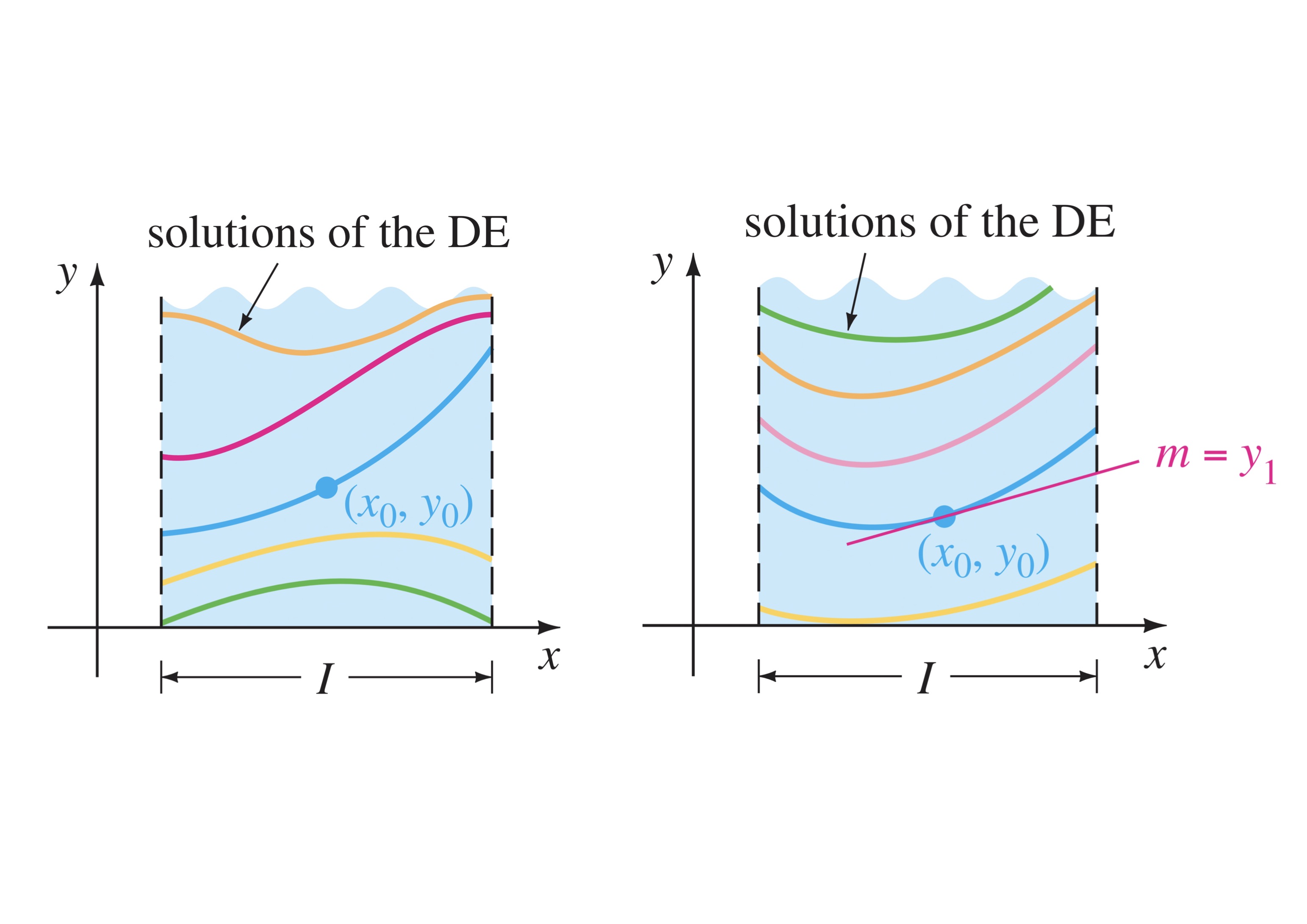
Remark. The words initial conditions derive from physical systems where the independent variable is time \(t\) and where \(y(t_0) = y_0\) and \(y'(t_0) = y_1\) represent the position and velocity, respectively, of an object at some beginning, or initial, time \(t_0\) (See your Mechanics course).

Examples

1. \(y'=3y, \quad \text{subject to} \quad y(0)=5.7\)

2. Revisited \(\dfrac{d^3 y}{dx^3}=\sin 2x+e^{-2x}+x^2+x+7, \quad \text{subject to} \quad y(0)=0,y'(0)=1,y''(0)=0\)

Try this for yourself based on the solution we have already obtained previously.

Notice from the above example that:

• We had a third order derivative and we needed three initial conditions in order to find specific values for the the three arbitrary constants, i.e. a particular solution. In other words, the order of the differential equation dictates how many initial conditions are required in order to find a particular solution.
  

3. \(\dfrac{d y}{dx}=-\dfrac{x}{y}, \quad \text{subject to} \quad y(4)=-3\)

4. \((e^{2y}-y) \cos x \dfrac{d y}{dx}=e^y \sin 2x, \quad \text{subject to} \quad y(0)=0\)

Exercise

In the problems below, find an explicit solution for the given initial-value problem.

1. \(\dfrac{d x}{dt}=4(x^2+1); \quad x(\pi/4)=1\)

2. \(\dfrac{d y}{dx}=\dfrac{y^2-1}{x^2-1}; \quad y(2)=2\)

3. \(x^2\dfrac{d y}{dx}=y-xy; \quad y(-1)=-1\)

Did you get it?

Check your understanding of some of the concepts covered at this stage by attempting the DYGIT? on Initial Value Problems. This is a formative assessment task and does not count for marks so please do it on your own to ascertain your own learning.

2.7 Systems of Linear First Order Ordinary Differential Equations (Self-Study Section)

This is a short self-study section. It is imperative that you work through this on your own to consolidate your understanding of this method. This method will come into effect once we study decay models in Chapter 3.

–> –> –> –> –>