Chapter 2 First-Order Differential Equations and Models

“Among all of the mathematical disciplines the theory of differential equations is the most important… It furnishes the explanation of all those elementary manifestations of nature which involve time.” - Sophus Lie (1842-1899) In Chapter 1 we built the conceptual machinery: what a model is, and why rates of change are the natural language for describing dynamic systems. This chapter is where Act I begins — we take that language and make it precise, and by the end of it you will have your first complete toolkit: the ability to take a first-order differential equation from unfamiliar symbols all the way to a solved, interpreted family of solutions.

The route runs as follows. First, we pin down exactly what a differential equation is and learn to classify one — by order, linearity, homogeneity, and coefficients — because classification is a diagnosis: it tells you which solution method to reach for. Next, we make precise what a solution even means, and how to verify whether a proposed function actually is one. Then, before solving anything at all, we learn to see the qualitative behaviour of every solution at once using a direction field. Finally, we develop our first two solution methods — direct integration and separation of variables — and use initial conditions to pin down the one particular solution a real problem demands.

One part of that route deserves special mention. Most students expect a differential equations course to be about solving equations, and it partly is. But some of the most powerful things you can do with a differential equation require no solving whatsoever, and the direction field is your first taste of that.

2.1 Differential Equations and Ordinary Differential Equations

Before we construct and solve any models, we need to pin down what an ordinary differential equation is, how we classify them, and hence which methods of solution apply. Some definitions first.

Remark. At this stage, I want to emphasize that you are registered for a degree in the mathematical sciences. You should not be afraid to grapple with technical and theoretical mathematical definitions. It is a key toolkit within your arsenal that you need to develop. If you have discomfort trying to decipher a mathematical definition, that is okay. However, you need not shy away from doing so, but instead try to make meaning that links the theory to the concepts. There is an inherent discomfort to learning. You also need to develop an aptitude for reading with comprehension. *rant over*

Definition 2.1 (Differential Equation) A differential equation (DE) is a mathematical equation that relates a function with its derivatives.

Definition 2.2 (Ordinary Differential Equation) An ordinary differential equation (ODE) is an equation that involves some ordinary derivatives of one or more unknown function (the dependent variable(s)) of one single independent variable.

For example: \[\begin{equation} \dfrac{d^2 y}{dx^2}+3\dfrac{d y}{dx}+2y=\sin{x} \tag{2.1} \end{equation}\]

Definition 2.3 (Partial Differential Equation) In contrast, a partial differential equation is an equation that involves some partial derivatives of one or more unknown function (the dependent variable(s)) of two or more independent variables.

For example: \[\begin{equation} \dfrac{\partial^2 u}{\partial x^2}+ \dfrac{\partial^2 u}{\partial y^2}=0 \end{equation}\]

Everything we do in this course involves ordinary differential equations only — one independent variable. From here on, differential equation and DE mean ordinary differential equation. You will meet partial differential equations in later years, once you have a firmer grasp of multivariable calculus.

Differential equations arise from many sources, and the independent variable can signify many different things. In these notes we use a variety of letters for the independent variable (including time \(t\)). Very often, though, the independent variable represents time, and the dependent variable is some dynamical quantity that depends on it.

2.2 Notation

Throughout these notes, ordinary derivatives will be denoted with the use of either the Leibniz notation, the prime notation, or Newton’s dot notation. Newton’s dot notation is most commonly used in physics, and it is mostly, but not exclusively, used to represent change with respect to time \(t\).

2.3 Classification of an Ordinary Differential Equation

Consider the general ordinary differential equation given below,

\[\begin{equation} a_{n}(x)\dfrac{d^n y}{dx^n}+a_{n-1}(x)\dfrac{d^{n-1} y}{dx^{n-1}}+\dots+ a_{2}(x)\dfrac{d^2 y}{dx^2}+a_{1}(x)\dfrac{d y}{dx}+a_{0}(x)y=g(x) \tag{2.2} \end{equation}\] where the coefficient functions, \(a_{n}(x), a_{n-1}(x), \dots, a_{2}(x), a_{1}(x), g(x)\) can be any functions of the independent variable \(x\) (including a constant/zero function).

We want to distinguish the ODEs that arise from this general form by their constituent features. The four classifications we use are:

2.3.1 Order

2.3.2 Linearity

2.3.3 Homogeneity

2.3.4 Coefficients

Remark. Why classify at all? Because classification is a diagnosis. Once you can classify a given ODE by these four features, you know which solution methods are available for it — exactly the way a doctor’s diagnosis determines the treatment. Whenever you face an unfamiliar differential equation, classification is always your first step. It may seem unnecessary now, but every solution method later in this chapter begins with the words “for an equation of this classification…”

2.3.1 Classification by order

Definition 2.4 (Order of an Ordinary Differential Equation) The order of a differential equation is the order of the highest derivative in the differential equation.

The order of Equation (2.1) is \(2\) or it is of the \(2\)nd order. This corresponds to the term with the highest derivative operator \(\dfrac{d^2 y}{dx^2}\).

The order of Equation (2.2) is \(n\) or it is of the \(n\)th order. This corresponds to the term with the highest derivative operator \(\dfrac{d^n y}{dx^n}\).

2.3.2 Classification by linearity

Definition 2.5 (Linearity of an Ordinary Differential Equation) A linear differential equation is one in which neither the unknown function nor any of its derivatives are raised to a power greater than 1.

An \(nth\)-order ODE such as in Equation (2.2) is said to be linear if

• the dependent variable (in this case, \(y\)) and all of its derivatives are of the first degree, that is, the power of each term involving the dependent variable \(y\) is 1, and
• the coefficients of the dependent variable \(y\) and any of its derivatives are constants, or they depend on the independent variable (in this case, \(x\)) only.

A differential equation that is not linear is said to be non-linear and this occurs when the above does not hold, that is, non-linear functions of the dependent variable or any of its derivatives occur in the differential equation.

Equation (2.1) is linear as \(\dfrac{d^2 y}{dx^2}, \dfrac{d y}{dx},\) and \(y\) are of the first degree, and its coefficients are all constants (1, 3, and 2 respectively). \(\sin{x}\) is non-linear in the independent variable, and thus has no effect on the linearity of Equation (2.1).

2.3.3 Classification by homogeneity

Definition 2.6 (Homogeneity of an Ordinary Differential Equation) A differential equation is homogeneous with respect to the dependent variable (say \(y\), in this case) if replacing the dependent variable with a non-zero arbitrary constant multiplied by the dependent variable does not change the structure of the differential equation. We say that the differential equation remains invariant under this transformation.

Otherwise, the differential equation is said to be non-homogeneous with respect to the dependent variable (in this case, \(y\)).

Otherwise stated, the ODE is homogeneous in the dependent variable if the substitution of \(ky\) (where \(k\) \(\neq\) 0) for \(y\) in the differential equation does not change the ODE. We will refer to this as the test for homogeneity. Any ODE that changes upon implementing the test will be classified as non-homogeneous.

We now implement the test for homogeneity on Equation (2.1) to check if this equation is homogeneous or not. To do this, let \(y=ky\), and so Equation (2.1) becomes \[\begin{equation} \dfrac{d^2 (ky)}{dx^2}+3\dfrac{d (ky)}{dx}+2ky=\sin{x}, \end{equation}\] \[\begin{equation} k\dfrac{d^2 y}{dx^2}+3k\dfrac{d y}{dx}+2ky=\sin{x}, \end{equation}\] \[\begin{equation} k\left( \dfrac{d^2 y}{dx^2}+3\dfrac{d y}{dx}+2y\right) =\sin{x}, \end{equation}\] \[\begin{equation} \dfrac{d^2 y}{dx^2}+3\dfrac{d y}{dx}+2y=\frac{1}{k}\sin{x}. \tag{2.3} \end{equation}\] Recall that \(k\) is a non-zero constant, i.e. \(k\neq 0.\) Thus, we can conclude that Equation (2.1) is non-homogeneous as the structure of the original Equation (2.1) and the resultant transformed Equation (2.3) are different.

Now, let us remove \(\sin{x}\) in Equation (2.1) to get the equation \[\begin{equation} \dfrac{d^2 y}{dx^2}+3\dfrac{d y}{dx}+2y=0. \tag{2.4} \end{equation}\] Let us now conduct the test for homogeneity on Equation (2.4). Again we let \(y=ky\) to get, \[\begin{equation} \dfrac{d^2 (ky)}{dx^2}+3\dfrac{d (ky)}{dx}+2ky=0, \end{equation}\] \[\begin{equation} k\dfrac{d^2 y}{dx^2}+3k\dfrac{d y}{dx}+2ky=0, \end{equation}\] \[\begin{equation} k\left( \dfrac{d^2 y}{dx^2}+3\dfrac{d y}{dx}+2y\right) =0, \end{equation}\] Since \(k \neq 0\), it follows that \[\begin{equation} \dfrac{d^2 y}{dx^2}+3\dfrac{d y}{dx}+2y=0 \tag{2.5} \end{equation}\] Equation (2.4) is homogeneous as it is the same as Equation (2.5) under the transformation, i.e. the equation remained invariant.

Let us now clarify or refine this definition for homogeneity for linear ordinary differential equations.

Definition 2.7 (Homogeneity of a Linear Ordinary Differential Equation) Consider the \(nth\)-order linear ODE given in Equation (2.2). \[\begin{equation} a_{n}(x)\dfrac{d^n y}{dx^n}+a_{n-1}(x)\dfrac{d^{n-1} y}{dx^{n-1}}+\dots+ a_{2}(x)\dfrac{d^2 y}{dx^2}+a_{1}(x)\dfrac{d y}{dx}+a_{0}(x)y=g(x) \tag{2.2} \end{equation}\] where the coefficient functions, \(a_{n}(x), a_{n-1}(x), \dots, a_{2}(x), a_{1}(x), g(x)\) can be any functions of the independent variable \(x\) (including a constant/zero function).

Equation (2.2) is non-homogeneous with respect to the dependent variable (say \(y\), in this case) if \(g(x) \neq 0\), in other words \(g(x)\) is not identically zero and the ODE contains terms that are functions of the independent variable, including constants.

Now consider the case when \(g(x)=0\), that is \[\begin{equation} a_{n}(x)\dfrac{d^n y}{dx^n}+a_{n-1}(x)\dfrac{d^{n-1} y}{dx^{n-1}}+\dots+ a_{2}(x)\dfrac{d^2 y}{dx^2}+a_{1}(x)\dfrac{d y}{dx}+a_{0}(x)y=0 \tag{2.6} \end{equation}\] An \(nth\)-order linear ODE such as in Equation (2.6) is homogeneous with respect to the dependent variable (say \(y\), in this case) if \(g(x)=0\), in other words it does not contain any term that is a function of the independent variable only, including constants.

Based on the above refined definition for homogeneity for linear ODEs, Equation (2.1) is a non-homogeneous second-order linear ordinary differential equation since \(g(x)=\sin x\) (a non-zero function of the independent variable \(x\)), whereas Equation (2.4) is a homogeneous second-order linear ordinary differential equation since \(g(x)=0\).

Remark. One can only use Definition 2.7 for homogeneity once you have concluded that the ODE is linear. In that case, homogeneity can be done by inspection based on whether the function of the independent variable \(g(x)=0\) (homogeneous) or \(g(x) \neq 0\) (non-homogeneous).

To summarize: the key difference between homogeneous and non-homogeneous linear ODEs is the presence of a forcing term. In a non-homogeneous linear ODE, there is an additional term which is not identically zero: a function (on the right-hand side) that depends on the independent variable, such as \(f(x)\) or \(g(t)\). This function is called the forcing term or the non-homogeneous part of the equation because it forces the solution to have a particular behaviour. Non-homogeneous ODEs are used to model phenomena where there is an external influence on the system being modeled, such as in electrical circuits or mechanical systems.

In contrast, a homogeneous linear ODE is an equation in which the forcing term is identically zero. Homogeneous ODEs are used to model phenomena where the system being modeled is self-contained and does not have any external influences. An example of a homogeneous ODE is \(y'' + 4y' + 3y = 0\), where \(y=y(x)\), which models the behavior of a mass-spring system without any external forces acting on it.

2.3.4 Classification by coefficients

Definition 2.8 (Coefficients of an Ordinary Differential Equation) The coefficient of any term of an ODE is that factor of the term which does not involve the unknown function or any of its derivatives. An ODE can have constant or variable (non-constant) coefficients.

An ODE has constant coefficients if all terms in the equation involving the dependent variable and its derivatives are preceded by coefficients that are constants.

An ODE has variable coefficients if at least one of the terms in the equation involving the dependent variable and its derivatives are preceded by coefficients that are functions of the independent variable.

Equation (2.1) has constant coefficients. The coefficients of \(\dfrac{d^2 y}{dx^2}\) is 1, \(\dfrac{d y}{dx}\) is 3, and \(y\) is 2, all of which are constants.

The coefficients play a crucial role in determining the behavior of the solution to an ODE. They can affect whether the solution is oscillatory or decaying, and they can also impact the stability of the solution. Understanding the coefficients is essential for solving and interpreting ODEs.

Classification at a glance

The figure below summarises the four questions you ask of any ODE. Work through them in order, every time.

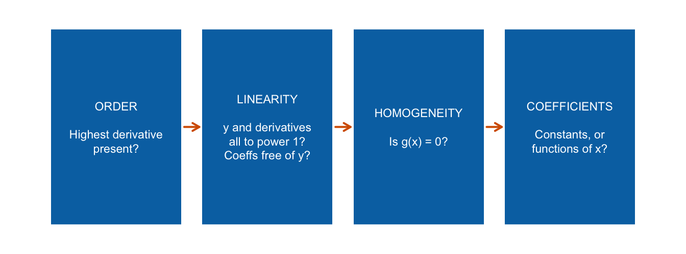
Figure 2.1: The four classification questions, asked in order.

Classification of Differential Equations: Examples

1. \(\dfrac{d^2 y}{dx^2}-2\dfrac{d y}{dx}+3y=0\)

2. \(5 \dfrac{d^2 x}{dt^2}+7\dfrac{d x}{dt}-8x=e^{x}\)

3. \(x^2\dfrac{d^2 y}{dx^2}+x\dfrac{d y}{dx}-y=0\)

4. \(s\dfrac{d^3 s}{dt^3}-6\left( \dfrac{d^2 s}{dt^2}\right) ^2+3\dfrac{d s}{dt}=0\)

Exercise:

Check if the following differential equations are ODEs, and then classify them in terms of their order, linearity, homogeneity, and coefficients:

1. \(t \dfrac{d^3 x}{dt^3}-2\left(\dfrac{d x}{dt}\right) ^4+x=0\)

2. \(y y'+2y=1+x^2\), where \(y=y(x)\)

3. \(y''+9y=\sin y\), where \(y=y(x)\)

4. \(\dfrac{d^2 R}{dt^2}=\dfrac{\kappa}{R^2}\), where \(\kappa\) (read: kappa) is a constant

5. \(x^5\dfrac{d^4 y}{dx^4}-x^3 \dfrac{d^3 y}{dx^3}+6y=0\)

6. \(\dfrac{d^2 x}{dt^2}=\sqrt{1+\left( \dfrac{d x}{dt}\right) ^2}\)

Did you get it?

Check your understanding of some of the concepts covered at this stage by attempting the DYGIT? on ODEs and Classification. This is a formative assessment task and does not count for marks so please do it on your own to ascertain your own learning.

2.4 Solutions of Ordinary Differential Equations

Differential equations appear naturally in mathematics and physics as the determining equations governing the behaviour of physical systems. The key outcome of this chapter is to find solutions to the various classes of differential equations that arise from our modelling processes.

Recall the fundamental contrast from Chapter 1: the solution to an algebraic equation is a number; the solution to a differential equation is a function. The solution to a continuous model is therefore not a snapshot of what a system is doing at one moment (static), but a description of how the system evolves (dynamic). The particular behaviour at a given point can then be found by evaluating the solution function at that point.

2.4.1 Concept of a Solution

Definition 2.9 (Solution of an Ordinary Differential Equation) A function \(y=h(x)\) is a solution of a given \(n\)-th order differential equation in the unknown dependent variable \(y\) and the independent variable \(x\) if it is defined on some interval \(I\), and identically satisfies the differential equation for all \(x\) in \(I\).

In other words, substituting \(y=h(x)\) into the differential equation reduces the equation to an identity. We say that \(y=h(x)\) satisfies the differential equation.

Remark. A caution for completeness: it would be incorrect to assume that every differential equation possesses a solution. The existence and uniqueness of solutions is its own body of theory, which you will meet properly in later courses. We flag it here so that “does a solution even exist?” stays on your radar as a legitimate mathematical question.

Verification of a Solution

To verify that a given function \(y=h(x)\) is a solution: substitute it into both sides of the DE separately, and check that the two sides produce the same expression for every \(x\) in the interval \(I\). This is a skill you already fully possess — it needs only differentiation and algebra, no solution methods at all.

Example: Verify that \(y=\frac{1}{16}x^4\) is a solution to the DE \(\dfrac{d y}{dx}=xy^{\frac{1}{2}}\)

Solution:

1. Remark (A reliable verification recipe).
2. Compute every derivative of \(h(x)\) that appears in the DE.
3. Substitute \(h(x)\) and its derivatives into the left-hand side only, and simplify fully.
4. Substitute into the right-hand side only, and simplify fully.
5. Compare. If the two simplified expressions are identical for all \(x \in I\), then \(h\) is a solution on \(I\). If they differ for even one \(x\) in \(I\), it is not.

The most common error is substituting into both sides at once and manipulating the equation as if the conclusion were already true. Keep the two sides separate until the final comparison.

Definition 2.10 (Trivial Solution of an Ordinary Differential Equation) A trivial solution of a differential equation is a solution that is identically zero on an interval \(I\).

Definition 2.11 (Explicit Solution of an Ordinary Differential Equation) An explicit solution of a differential equation is a solution \(y=h(x)\) in which the dependent variable is expressed solely in terms of the independent variable and constants.

Exercise:

Verify that the indicated function is a solution of the given differential equation on the interval \((-\infty, \infty)\).

1. \(y''-2y'+y=0; \quad y=xe^x\)
2. \(u''(t)+2u'(t)+2u(t)=0;\)
   • 1. \(\quad u(t)=e^{-t}\sin t,\)
   • 2. \(\quad u(t)=e^{-t}\cos t\)

Thinking Questions:

1. We do not yet know how to find the solutions to a DE. Based on the above exercise, given the solution to the DE, are you able to think of how we landed up with that solution?
2. In the second question in the exercise, two solutions are given. What does that tell you?
3. Do those two differential equations contain the trivial solution?

2.4.2 Solution Curves

Definition 2.12 (Solution Curve of an Ordinary Differential Equation) The solution curve of a differential equation is the graph of its solution \(y=h(x)\).

The study of differential equations is similar to that of integral calculus. When you evaluated an indefinite integral in calculus, you used a single constant \(c\) of integration. In the same way, when solving a first-order differential equation, we usually obtain a solution containing a single arbitrary constant or parameter \(c\).

Remark. We can use any letter or symbol to represent an arbitrary constant. There is no convention in this regard. Remember that the arbitrary constant is just a placeholder for the infinite number of solutions that the general solution to a differential equation possesses.

The number of arbitrary constants in a solution is governed by the order of the differential equation. Hence, a first-order differential equation will have a solution containing one arbitrary constant, whereas an \(n\)th-order differential equation will have a solution containing \(n\) arbitrary constants.

Definition 2.13 (General Solution of an Ordinary Differential Equation) The general solution of a differential equation is the solution that contains one or more arbitrary constants or parameters.

The arbitrary constant encompasses all the infinite solutions that the differential equation satisfies. A solution containing one arbitrary constant gives rise to a set of solutions called a one-parameter family of solutions. When solving an nth-order differential equation, we get an n-parameter family of solutions. This means that a single differential equation can possess an infinite number of solutions corresponding to the unlimited number of choices for the arbitrary constant(s)/parameter(s).

Definition 2.14 (Family of Solution Curves of an Ordinary Differential Equation) A family of solution curves of a differential equation is the geometric solution of a differential equation containing infinitely many solution curves, one for each value (or combination of values) of the arbitrary constants or parameters.

We may also be interested in a solution to the differential equation for a particular value(s) of the arbitrary constant(s).

Definition 2.15 (Particular Solution of an Ordinary Differential Equation) A particular solution of a differential equation is a solution that does not contain any arbitrary constants or parameters.

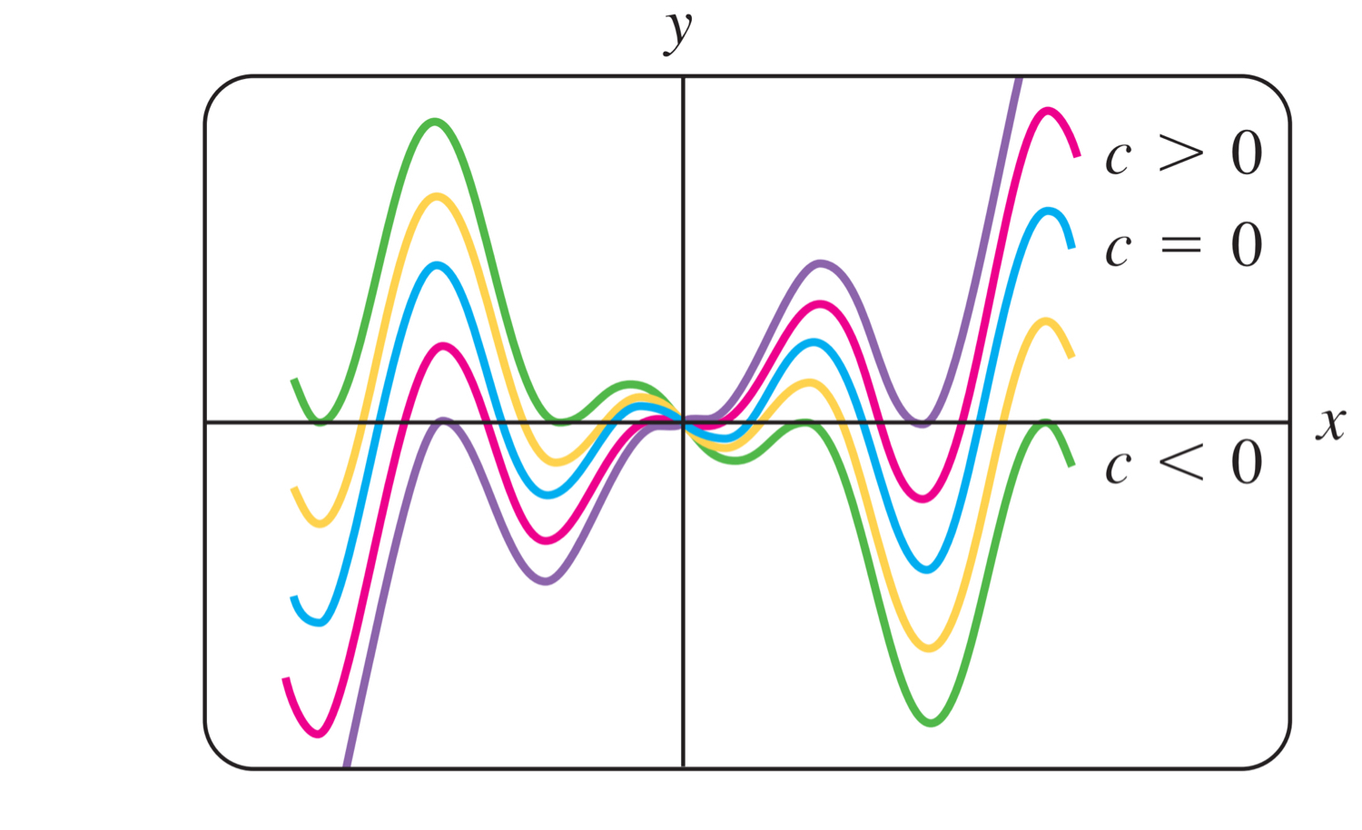
For example, the one-parameter family of solutions given by \(y=cx-x \cos x\) is an explicit solution of the linear first-order differential equation \(xy'-y= x^2 \sin x\) (Verify this). Figure 1 below taken from Zill and Cullen, shows the graphs of some of the solutions in this family governed by infinite values of the arbitrary constant \(c\). The solution \(y=-x \cos x\), the blue curve in the figure, is a particular solution corresponding to the value of the arbitrary constant \(c=0\).

Figure 1: A one-parameter family of solutions

Exercise:

Draw a rough sketch or use a graphing calculator like Desmos to find the family of solution curves for the following differential equations:

1. \(y'=\cos x; \quad y=\sin x + c\)
2. \(y'=-0.2y, \quad y=Be^{-0.2t}\)

Did you get it?

Check your understanding of some of the concepts covered at this stage by attempting the DYGIT? on Solutions of ODEs. This is a formative assessment task and does not count for marks so please do it on your own to ascertain your own learning.

2.4.3 Direction Fields: Seeing Solutions Without Solving

Here is a remarkable fact. Take any first-order differential equation in the form

\[\begin{equation} \dfrac{dy}{dx}=f(x,y) \tag{2.7} \end{equation}\]

We may not know how to solve it yet — but we can already draw a picture of every one of its solutions at once. The reason is hiding in plain sight: the equation itself tells us the slope of the solution curve at every point \((x,y)\) in the plane. If a solution curve passes through the point \((x, y)\), then at that point, its slope must equal \(f(x,y)\) — that is precisely what the differential equation says.

Definition 2.16 (Lineal Element) A lineal element at the point \((x,y)\) is a short line segment drawn through \((x,y)\) with slope \(f(x,y)\), representing the direction a solution curve of \(\frac{dy}{dx}=f(x,y)\) must travel as it passes through that point.

Definition 2.17 (Direction Field) A direction field (or slope field) of the differential equation \(\frac{dy}{dx}=f(x,y)\) is the collection of lineal elements drawn at each point of a grid covering some region of the \(xy\)-plane. It shows, at a glance, the direction in which every solution curve flows through that region.

Think of the direction field as a flow map: drop a leaf anywhere on it, and the lineal elements tell you where the current carries it. Each possible path of the leaf is one member of the family of solution curves — one particular solution for each starting point.

Reading a direction field

Consider the differential equation

\[\dfrac{dy}{dx} = x - y.\]

We have no method to solve this yet. But we can compute slopes: at the point \((0,0)\) the slope is \(0-0=0\) (flat); at \((2,0)\) the slope is \(2\) (steeply up); at \((0,2)\) the slope is \(-2\) (steeply down). Repeating this over a grid, and overlaying three particular solutions, gives:

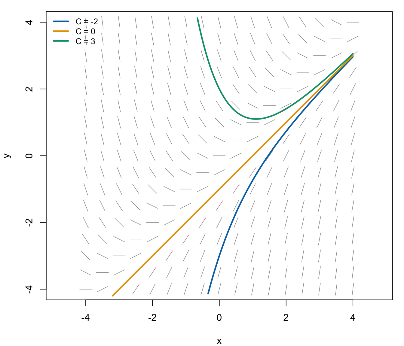
Figure 2.2: Direction field for \(dy/dx = x - y\), with three particular solution curves overlaid. Every solution curve is everywhere tangent to the lineal elements it passes through.

Study the figure and notice three things:

1. Every solution curve threads through the field, everywhere tangent to the lineal elements. The curves never cross the “grain” of the field.
2. The three curves differ only in their constant \(C\) — they are three members of the one-parameter family of solutions, each singled out by where it starts.
3. Long-run behaviour is visible without solving: every solution is eventually funnelled toward the line \(y = x - 1\). The direction field reveals this qualitative fact even if we never find the formula.

Remark. This is the first appearance of a theme that runs through the whole course: qualitative analysis. There are differential equations — many of the most important ones in science — that cannot be solved in closed form at all. For those equations, pictures like this are not a nice-to-have; they are the primary tool. When we reach systems of equations in Chapter ??, the two-dimensional cousin of the direction field (the phase portrait) will carry the entire analysis.

A second example: growth and decay foreshadowed

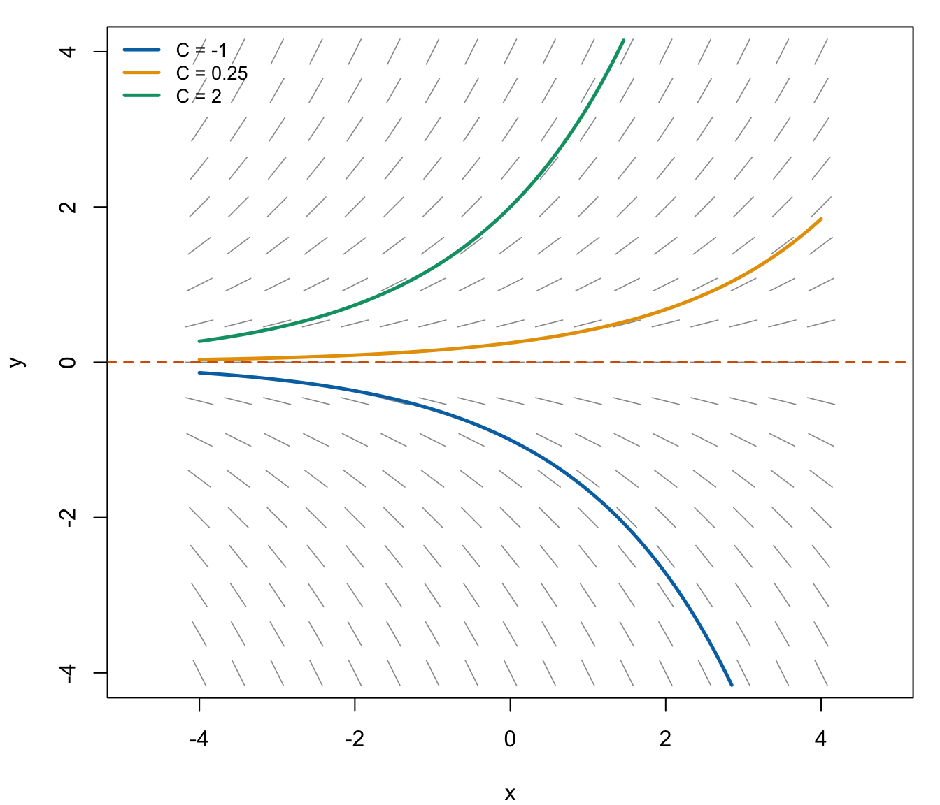
Figure 2.3: Direction field for \(dy/dx = 0.5\,y\). The slopes depend only on \(y\), so every horizontal line of lineal elements is identical — and solutions grow away from \(y=0\) exponentially.

Notice the dashed line \(y = 0\): the slope there is zero everywhere, so the constant function \(y=0\) is itself a solution — the trivial solution from Definition 2.10, sitting visibly inside the field. Solutions starting above it grow away upward; solutions below it grow away downward. When we build growth and decay models shortly, this picture is exactly what “exponential growth” looks like before we write down \(y = Ce^{kx}\).

Explore: the interactive direction field

Static pictures only go so far. Use the interactive field below: choose a differential equation, then click anywhere on the field to drop a starting point — the solution curve through that point is traced instantly. Click several points to build up the family of solutions with your own hands.

dy/dx = x − y 0.5 y −y x y sin(x) y(1 − y) Click the field to trace a solution through that point.

Try this with the widget:

1. With \(dy/dx = x - y\) selected, click five different starting points. Do all your curves eventually hug the same straight line? Which line?
2. Switch to \(dy/dx = y(1-y)\) (the logistic equation — a preview of population modelling). Click starting points at \(y \approx 0.1\), \(y \approx 0.5\), and \(y \approx 1.5\). What value does every positive solution approach? Now click a point with \(y < 0\). What happens, and why is this behaviour completely invisible if you only look at the equation’s formula?
3. Switch to \(dy/dx = \sin(x)\). The slopes here depend only on \(x\). What does that mean about how any two solution curves are related to each other? (Hint: think vertical shifts — and think about what “+ C” meant in integration.)

Exercise:

1. By hand, sketch the direction field of \(\dfrac{dy}{dx} = -\dfrac{x}{y}\) on the grid of integer points \(x, y \in \{-2, -1, 0, 1, 2\}\) (omit points where \(y = 0\)). What familiar family of curves do the solutions appear to form? Verify your guess by checking that \(x^2 + y^2 = c\) implicitly satisfies the DE.
2. Without solving, use a hand sketch or the widget to determine the long-run behaviour (\(x \to \infty\)) of solutions to \(\dfrac{dy}{dx} = -y\): what happens to every solution regardless of its starting point? What single feature of the direction field makes this obvious?
3. True or false, with a reason: two distinct solution curves of the same first-order differential equation \(\frac{dy}{dx}=f(x,y)\) (with \(f\) well-behaved) can cross each other at a point where the field is defined. What would the direction field have to look like at a crossing point?

Thinking Questions:

1. A direction field is built by evaluating \(f(x,y)\) at finitely many grid points, yet we use it to draw conclusions about all solutions at all points. What are we implicitly assuming about \(f\) for this to be trustworthy?
2. Both the direction field and the family-of-solution-curves picture (Section 2.4.2) display “all the solutions at once.” What is the key difference in what each requires you to know beforehand?

Did you get it?

Check your understanding of direction fields by attempting the DYGIT? on Direction Fields. (Link to be added once the quiz is created on Moodle.)

2.5 Methods of Solution for Ordinary Differential Equations

Euler’s Number and Ordinary Differential Equations

Before we develop our first solution methods, let us familiarize ourselves with some interesting aspects of the behaviour of an important function and its derivatives — a function that will appear, again and again, in the solutions that follow.

Let us consider the function \(y = e^{x}\). This function has many interesting characteristics. For example, consider its derivative, \[\begin{equation*} \dfrac{d}{dx} e^{x} =\lim_{h \to 0}{\dfrac{e^{x + h} - e^{x}}{h}}. \end{equation*}\] If we simply factor out the \(e^{x}\) and note it is not affected by the limit, we get the following, \[\begin{equation*} \dfrac{d}{dx}e^{x} = e^{x} \lim_{h \to 0}{\dfrac{e^{h} - 1}{h}}. \end{equation*}\] With a simple substitution of \(n = e^{h}-1\) and some algebraic manipulation we can show that this is equivalent to \[\begin{equation} \dfrac{d}{dx} e^{x} = e^{x}\dfrac{1}{\lim_{n \to 0}\ln{(1+n)^{\dfrac{1}{n}}}}. \tag{2.8} \end{equation}\] At this point we note that \[\begin{equation} e = \lim_{n \to 0}{(1+n)^{\dfrac{1}{n}}}, \tag{2.9} \end{equation}\] where both of these have an approximate solution of 2.7182818284… We call \(e\) Euler’s number. Now substituting Equation (2.9) into Equation (2.8), we find a useful result. \[\begin{equation} \dfrac{d}{dx} e^{x} = e^{x}. \end{equation}\] Using this knowledge we can consider evaluating the derivative of \[\begin{equation} y = \ln{x}. \tag{2.10} \end{equation}\] After a simple manipulation of Equation (2.10), we get \[\begin{equation*} e^{y} = x. \end{equation*}\] Applying implicit differentiation to this we get \[\begin{equation*} e^{y} \dfrac{dy}{dx} = 1. \end{equation*}\] Rearranging we find \[\begin{equation*} \dfrac{dy}{dx} = \dfrac{1}{e^{y}}. \end{equation*}\] By substituting Equation (2.10) into this we get \[\begin{equation*} \dfrac{dy}{dx} = \dfrac{1}{e^{\ln{x}}}, \end{equation*}\] which simplifies to our next useful result. \[\begin{equation*} \dfrac{d}{dx} \ln{x} = \dfrac{1}{x}. \end{equation*}\]

Remark. Pause on what we just found, because in a differential equations course it is the whole point: \(e^x\) is a function whose instantaneous rate of change is itself. In the language of this chapter, \(y = e^x\) is a solution of the differential equation \(y' = y\). In fact, this property essentially defines the exponential function — and it is precisely why \(e\) will appear in the solution of nearly every model of growth, decay, cooling, and oscillation in this course. Whenever a quantity’s rate of change is proportional to the quantity itself, \(e\) is already in the room.

We will start by considering the following these methods of solution for ordinary differential equations:

2.5.1 The Method of Direct Integration

2.5.2 The Method of Separation of Variables

These are just two analytical methods for finding solutions to differential equations. There are numerous other analytical and numerical methods you will encounter in Mathematics, Physics, and further studies in Applied Mathematics, some of which we will cover in later sections and chapters.

Before delving in to the Methods section, I would like to draw your attention back to the preceding Chapter on the Prerequisites for this course. It would be worthwhile digging out your Calculus notes now. Here is a quick preamble:

2.5.1 The Method of Direct Integration

The Method of Direct Integration can be used for \(n\)-th order differential equations, provided that they are differential equations that can be written in the standard form: \[\begin{equation} \dfrac{d^n y}{dx^n}=g(x). \tag{2.11} \end{equation}\]

Notice the following key classification criteria:

• The left hand side of the differential equation in (2.11) contains a single derivative of the dependent variable, of any order. The key here is that there are not multiple derivatives of the dependent variable.
• The derivative of the dependent variable is linear, meaning its degree is at most one, and there contains no products of the dependent variable with this derivative.
• The right hand side of the differential equation in (2.11) is a function of the independent variable only, i.e. \(g=g(x)\). This may include a constant/non-zero function of the independent variable. This means that the right hand side of the differential equation cannot contain any term or function involving the dependent variable.

If these classification criteria are met, the differential equation can be solved using the Method of Direct Integration. In this case, you can integrate the differential equation a sufficient number of times (\(n\) times in (2.11)) until \(y\) is found.

For example, the equation \[\begin{equation*} \dfrac{d^2 y}{dx^2}= x^3+3x+1, \end{equation*}\] satisfies the aforementioned criteria as the left hand side contains a single derivative of the dependent variable \(y\) that is linear and of the second order, while the right hand side contains some function of the independent variable \(x\). However, the equation \[\begin{equation} \dfrac{d x}{dt}= 3t+x^2, \end{equation}\] does not meet the criteria for the Method of Direct Integration. Even though the left hand side contains a single derivative of the dependent variable \(x\) that is linear and of the first order, the right hand side contains some function of the independent and dependent variable, i.e. \(g=g(t,x)\). What about the differential equation \[\begin{equation} y''+y'= x^3+3x+1, \end{equation}\] where \(y=y(x)\)? While the right hand side contains some function of the independent variable \(x\) only, the left hand side contains both a second and first derivative of the dependent variable, thus the Method of Direct Integration cannot be used here.

Remark. Please note here that a differential equation may not present itself in the form set out in Equation (2.11). Sometimes, manipulation will be required in order to write a given DE in this form before you can apply the method. But it is equally important that you do not force an equation to meet this form if it cannot be done. All that means is the differential equation cannot be solved using this method, and that another method may be applicable.

For example, do the following differential equations meet the criteria to use the Method of Direct Integration? \[\begin{equation} y''= x^3+3x-2y''+1, \tag{2.12} \end{equation}\] and \[\begin{equation} \left(\dfrac{d^2 y}{dx^2}\right)^{2}= x^3+3x+1. \tag{2.13} \end{equation}\]

Think about each of these before reading on.

For Equation (2.12), the answer is yes — after manipulation. The \(-2y''\) on the right looks disqualifying, but it is not a different derivative; collecting like terms gives \(3y'' = x^3+3x+1\), and hence \[\begin{equation*} y'' = \tfrac{1}{3}\left(x^3+3x+1\right), \end{equation*}\] which meets every criterion. This is exactly the manipulation the remark above anticipates: tidy first, classify second.

Equation (2.13) is different: as written, the second derivative appears to the second degree, violating the linearity criterion, so the method does not apply directly. (A thinking point for the curious: one could take square roots to obtain \(y'' = \pm\sqrt{x^3+3x+1}\) — each branch is in standard form on the region where the radicand is non-negative, but now there are two separate equations and domain restrictions to manage. The lesson: a degree greater than one is never harmless, even when a workaround seems available.)

Remark. It is important to remember the reasons why we were interested in classifying a differential equation. Hopefully you can see now how certain elements of classification are key markers to determine when a method of solution is applicable.

Once a given differential equation is shown to meet the form specified in Equation (2.11), the method of solution is simple: integrate both sides of the differential equation with respect to the independent variable \(x\), i.e. \[\begin{equation} \int \dfrac{d^n y}{dx^n} dx=\int g(x) dx, \end{equation}\] and repeat until \(y\) itself is recovered — \(n\) integrations in total.

Watch what the repeated integration does to the constants. The first integration produces one arbitrary constant, \(c_1\). The second integration integrates everything, including that constant, so \(c_1\) becomes \(c_1 x\) and a new constant \(c_2\) appears. After all \(n\) integrations, the general solution has the form \[\begin{equation} y=G(x)+c_1x^{n-1}+c_2x^{n-2}+\dots+c_{n-1}x+c_{n}, \tag{2.14} \end{equation}\] where \(G(x)\) is an \(n\)-fold antiderivative of \(g(x)\), and \(c_1, c_2, \dots, c_n\) are arbitrary constants (any numerical factors, such as the \(\frac{1}{2}\) that arises from integrating \(c_1x\), are absorbed into the arbitrary constants). Equation (2.14) represents the general solution of the differential equation (2.11) by using the Method of Direct Integration.

Remark. Notice the count: an \(n\)-th order equation, \(n\) integrations, \(n\) arbitrary constants — an \(n\)-parameter family of solution curves, exactly as we saw in Section 2.4.2. Notice also that the constants do not simply pile up as \(c_1 + c_2 + \dots\) (that sum would collapse into a single constant!); the repeated integration spreads them across a polynomial of degree \(n-1\), and it is this polynomial structure that makes the \(n\) constants genuinely independent of one another.

Let us look at a simple first order case. This is what I mean:

Let us now consider some examples:

Examples

1. \(\dfrac{d y}{dx}+\sin 2x=0\)

2. \(\dfrac{d^3 y}{dx^3}=\sin 2x+e^{-2x}+x^2+x+7\)

Notice from the above example that:

• We had a third order derivative and we needed to integrate three times to find the solution for the dependent variable \(y\). In other words, the order of the differential equation dictates how many integrations you need to do.
• These three integrations resulted in three arbitrary constants. In other words, the order of the differential equation will dictate the parameter of the family of solution curves.
• When integrating the differential equation the second and third time, it is imperative that you remember to integrate the terms containing any arbitrary constant as well — this is precisely how the polynomial in Equation (2.14) arises.
• Be wary of your signs when integrating.

Did you get it?

Check your understanding of some of the concepts covered at this stage by attempting the DYGIT? on Direct Integration. This is a formative assessment task and does not count for marks so please do it on your own to ascertain your own learning.

2.5.2 The Method of Separation of Variables

Unlike the Method of Direct Integration outlined in 2.5.1, the Method of Separation of Variables can only be used for first-order differential equations. In exchange for that restriction, it buys us something direct integration could not: the right hand side is now allowed to involve the dependent variable — provided it does so in a very particular way.

Consider a first-order differential equation of the form \[\begin{equation} \dfrac{d y}{dx}=g(x)h(y). \tag{2.15} \end{equation}\]

Notice the following key classification criteria:

• The left hand side of the differential equation in (2.15) contains a single derivative of the dependent variable that is of the first order. The key here also is that there are not multiple derivatives of the dependent variable, only the first derivative.
• The first derivative of the dependent variable is linear, meaning its degree is at most one.
• The right hand side of the differential equation in (2.15) consists of the product of distinct functions of the dependent variable \(y\) and the independent variable \(x\), i.e. it contains a separate and distinct product of functions \(g=g(x)\) and \(h=h(y)\). Here also, the functions \(g\) and \(h\) may include a constant/non-zero function of the dependent or independent variable respectively. This means that the right hand side of the differential equation may contain terms or functions involving the dependent variable, provided it is a product with the terms or functions involving the independent variable.

If these classification criteria are met, the differential equation can be solved using the Method of Separation of Variables. For example, the equation \[\begin{equation*} \dfrac{d y}{dx}= y^2 x e^{3x+4y}, \end{equation*}\] is separable as it satisfies the aforementioned criteria as the left hand side contains a single first derivative of the dependent variable \(y\) that is linear and of the first order, while the right hand side contains a product of a function of the independent variable (\(g(x)=xe^{3x}\)), and a function of the dependent variable (\(h(y)=y^2e^{4y}\)). Notice that some manipulation was required here — the key step is recognising that \(e^{3x+4y} = e^{3x}e^{4y}\) factors, which is what allows the split. However, the equation \[\begin{equation} \dfrac{d x}{dt}= x +\sin t, \end{equation}\] is not separable as it does not meet the criteria for the Method of Separation of Variables. Even though the left hand side contains a single derivative of the dependent variable \(x\) that is linear and of the first order, there is no way of expressing the right hand side \(x +\sin t\) as a product of a function of the independent variable \(t\) (\(g(t)\)), and a function of the dependent variable \(x\) (\(h(x)\)). Try your best :)

Remark. A useful rule of thumb: sums across the variables break separability; products preserve it. The expression \(x + \sin t\) is a sum mixing both variables — unsalvageable. The expression \(y^2xe^{3x+4y}\) looks worse but is secretly a pure product. When in doubt, attempt the factorisation explicitly and see whether every \(x\) lands in one factor and every \(y\) in the other.

Remark. Please note again here that a differential equation may not present itself in the form set out in Equation (2.15). Sometimes, manipulation will be required in order to write a given DE in this form before you can apply the method. But it is equally important that you do not force an equation to meet this form if it cannot be done. All that means is the differential equation cannot be solved using this method, and that yet another method may be applicable.

Such a differential equation as written in the form given in Equation (2.15) is called separable since it is possible to separate the dependent and independent variables on different sides of the equation, i.e. \[\begin{equation*} \dfrac{1}{h(y)} \dfrac{d y}{dx}=g(x). \end{equation*}\] Under these specific circumstances when we have a first derivative only, we can treat the differentials/infinitesimals \(dy\) and \(dx\) as normal algebraic quantities and multiply or divide them on either side of the equation. This means that we can separate the dependent and independent variables on different sides of the equation along with its associated differential, i.e. \[\begin{equation*} \dfrac{1}{h(y)} dy=g(x) dx. \end{equation*}\] Once we have isolated the functions of the dependent variable \(y\) and its associated differential \(dy\), and the functions of the independent variable \(x\) and its associated differential \(dx\) on either side of the equation, we can then integrate both sides of the equation with respect to its associated differential, i.e. \[\begin{equation*} \int \dfrac{1}{h(y)} dy=\int g(x) dx. \end{equation*}\] We can then use the rules of integration as well as some algebraic manipulation in order to find a solution for the dependent variable \(y\). Hence, the general solution of Equation (2.15) is given by \[\begin{equation*} \int \dfrac{1}{h(y)} dy=\int g(x) dx +c, \end{equation*}\] where \(c\) is the constant of integration. Note here that even though we are computing an integral on either side of the equation, we only require one constant of integration due to the nature of arbitrary constants.

Remark (Watch for the solutions you divide away). The very first move of this method — dividing by \(h(y)\) — silently assumes \(h(y) \neq 0\). But any constant value \(y = y_0\) with \(h(y_0)=0\) makes the right hand side of Equation (2.15) zero, and a constant function has zero derivative — so each such \(y = y_0\) is a perfectly good solution of the differential equation that the division step discards. Before you divide, note the zeros of \(h\); after you solve, check whether each of these constant solutions is recovered by some value of your arbitrary constant, and if not, state it separately alongside the general solution.

You have, in fact, already met these constant solutions: they are exactly the horizontal lines of flat lineal elements you saw in Section 2.4.3 — the ones every nearby solution funnels toward or away from. The logistic equation \(y'=y(1-y)\) in the interactive widget has two of them, \(y=0\) and \(y=1\); try to spot them in its field.

Let us see this subtlety play out in full on the simplest interesting example. Consider \[\begin{equation*} \dfrac{dy}{dx} = xy. \end{equation*}\] The zeros of \(h(y) = y\) tell us immediately that the constant function \(y = 0\) is a solution (check: both sides vanish). For \(y \neq 0\) we separate and integrate: \[\begin{equation*} \int \dfrac{1}{y}\,dy = \int x\, dx \quad\Longrightarrow\quad \ln|y| = \dfrac{x^2}{2} + c. \end{equation*}\] Exponentiating both sides gives \(|y| = e^{c}e^{x^2/2}\), and hence \(y = \pm e^{c} e^{x^2/2}\). Since \(c\) is arbitrary, the quantity \(\pm e^{c}\) ranges over every nonzero real number, so we absorb it into a single new arbitrary constant \(C = \pm e^c \neq 0\): \[\begin{equation*} y = Ce^{x^2/2}. \end{equation*}\] Finally, notice that allowing \(C = 0\) in this formula recovers exactly the constant solution \(y=0\) we set aside at the start. So the complete general solution is \(y = Ce^{x^2/2}\) with \(C \in \mathbb{R}\) — one clean formula, but only because we checked. This absorb-and-recover pattern (\(\ln|y|\), exponentiate, fold \(\pm e^c\) into \(C\), then test \(C=0\)) recurs constantly in this course; make it a habit rather than a surprise.

Remark. It is important to note here that a separable ordinary differential equation may not necessarily be analytically solvable as the resulting integrals may not always be reducible to elementary functions.

Even when this integration is analytically possible, it is oftentimes the case that this solution for the dependent variable \(y\) will be in implicit form. We will endeavour as much as possible to write this solution in explicit form as outlined in Definition 2.11. Again, do not force a solution into explicit form if it cannot be written as such. We will leave such solutions in implicit form. If a question does not state otherwise, you can assume that I require an explicit solution. When an implicit solution is deemed sufficient, I will state that “you may leave your solution in implicit form”.

Examples

1. \(\dfrac{d y}{dx}=2\)

2.  \(\dfrac{d y}{dx}=\sin x\)

3.  \(\dfrac{d y}{dx}=xy\)

4.  \(\dfrac{d y}{dx}-2y=0\)

Try this on your own

5.  \(\dfrac{d y}{dx}-2y=3\)

(Ignore the reference in the beginning to page numbers and notes. This is my video from last year.)

6.  \(\dfrac{d y}{dx}-\dfrac{y}{x}=0\)

Try this on your own

7.  \(\dfrac{d y}{dx}-2y^2+5y=3\)

This example requires a full understanding of the algebraic technique called partial fraction decomposition which you have covered in Mathematics.

Thinking Questions:

1. Can a given differential equation meet the criteria to be solved by using either the Method of Direct Integration, or the Method of Separation of Variables?
2. If so, what does that tell you?
3. If so, can you think of examples of such differential equations?
4. If so, go back to all the examples of differential equations you have seen thus far, and observe them through this dual lens.
5. In Examples 3 and 4 above, identify the constant solution that the division step temporarily discards, and confirm that it is recovered by the arbitrary constant in your final answer. Then find it as a horizontal line of flat lineal elements in the corresponding direction field.

Exercise

In the problems below, solve the given differential equation for its general solution in explicit form by using either the method of direct integration, separation of variables, or both. Where the method of separation of variables requires division by a function of the dependent variable, identify any constant solutions and state whether your final general solution recovers them.

1. \(\dfrac{d^2 x}{dt^2}+16x=0\)

2. \(\dot x+5x=10\)

3. \(\dfrac{d^3 y}{dx^3}-2y=0\)

4. \(y\dfrac{d y}{dx}=\sin 5x\)

5. \(\dfrac{d^3 y}{dx^3}=\sin 5x\)

6. \((1+x) dy-y dx=0\), where \(y=y(x)\)

7. \(\dfrac{d y}{dx}=(x+1)^2\)

8. \(dx+e^{3x}dy=0\), where \(y=y(x)\)

9. \(\dfrac{d^3 y}{dx^3}-2y^2=0\)

10. \(\dfrac{d^3 y}{dx^3}-2x^2=0\)

11. \(\dfrac{d S}{dt}-\dfrac{5S}{t}=0\)

12. \(y\dfrac{d y}{dx}=3y^2+1\)

13. \(y'-3y^2-y=0\)

14. \(\dfrac{d x}{dt}-x^2=-4\)

15. \(t \dot x -(1+t)x=0\)

16. \((a^2-x^2)y'+xy=0\), where \(a\) is a constant

17. \(\dfrac{d y}{dx}-\dfrac{y+3}{x^2-3x+2}=0\)

18. Find an implicit general solution to the following equation \(\dfrac{y}{x^2}\dfrac{d y}{dx}+e^{2x^{3}+y^{2}}=0\)

Did you get it?

Check your understanding of some of the concepts covered at this stage by attempting the DYGIT? on Separation of Variables. This is a formative assessment task and does not count for marks so please do it on your own to ascertain your own learning.

2.6 Initial Value Problems

Everything we have solved so far has produced a family: a general solution with one arbitrary constant per order of the equation. But no real modelling question ever wants the whole family. The coffee on your desk started at one particular temperature; the population being studied had one particular size when observation began. In the language of our modelling cycle, the formulate step gives us the differential equation — and the observed starting state of the system gives us the extra information that picks out the one member of the family that describes our situation. This section is about that final selection step.

As we have noted previously, the solution of an ordinary differential equation is not unique, as it contains arbitrary constants. This is a natural reflection of the fact that a physical law describes an infinitely large number of processes, hence an infinitely large number of solution curves. We had referred to this solution as the general solution. In order to obtain a unique process, or a unique solution of a differential equation, we need to use additional conditions that specify the initial state of the process. We refer to this solution as a particular solution.

We are often interested in problems in which we seek a solution \(y(x)\) of a differential equation so that \(y(x)\) satisfies these prescribed additional conditions imposed on the unknown function \(y(x)\) or any of its derivatives. That is, we need to

Solve: \[\begin{equation} \dfrac{d^n y}{dx^n}=f(x,y,y',...,y^{(n-1)}), \tag{2.16} \end{equation}\] Subject to: \[\begin{equation} y(x_0)=y_0, y'(x_0)=y_1,...,y^{(n-1)}(x_0)=y_{n-1}, \tag{2.17} \end{equation}\] where \(y_0\), \(y_1\),…,\(y_{n-1}\) are arbitrarily specified real constants, is called an nth-order initial-value problem (IVP) or Cauchy problem. The values of \(y(x)\) and its first \(n-1\) derivatives at a single point \(x_0\), as given in Equation (2.17), are called initial conditions.

Solving this nth-order initial-value problem entails first finding an \(n\)-parameter family of solutions of the given differential equation in Equation (2.16) (the general solution), and then using the \(n\) initial conditions at \(x_0\) in Equation (2.17) to determine numerical values of the \(n\) constants in the family (a particular solution). It is important to note here that the number of initial conditions coincides with the order of the differential equation. So in this case, we have \(n\) initial conditions corresponding to an \(nth\) order differential equation. Otherwise stated, the number of initial conditions that need to be specified is equal to the number of arbitrary constants in the general solution.

Remark. The initial conditions must and can only be applied once the general solution has been found. A very common error is to impose the condition on an intermediate line of working — for instance, immediately after integrating one side of a separable equation — before the general solution is complete. Solve fully first; substitute the conditions last.

A first-order explicit ODE has an initial value problem that is of the form

Solve: \[\begin{equation} y'=f(x,y), \quad \text{subject to} \quad y(x_0)=y_0. \tag{2.18} \end{equation}\]

In most cases the unique solution of a given first-order initial value problem as given in Equation (2.18), hence a particular solution, is obtained from a general solution by an initial condition \(y(x_0)=y_0\), with given values \(x_0\) and \(y_0\), that is used to determine a value of the arbitrary constant \(c\). Geometrically this condition means that the solution curve should pass through the point \((x_0, y_0)\) in the \(xy\)-plane.

Remark (You have already done this with your mouse). If the geometric meaning feels abstract, you have in fact already performed it, physically, in Section 2.4.3: every time you clicked a point in the interactive direction field widget, you imposed an initial condition. The click chooses \((x_0, y_0)\); the traced curve is the particular solution of the corresponding IVP. And recall the observation from that section that solution curves of a well-behaved first-order equation never cross: this is precisely why one point suffices to pin down one curve — if two different particular solutions could pass through the same point, an initial condition could never single one out.

A second-order initial-value problem is of the form

Solve: \[\begin{equation} y''=f(x,y,y'), \quad \text{subject to} \quad y(x_0)=y_0, y'(x_0)=y_1. \tag{2.19} \end{equation}\] In geometric terms, we want to find a solution \(y(x)\) to the second-order initial value problem as given in Equation (2.19) so that its solution curve not only passes through \((x_0, y_0)\), but the slope of the curve at this point is the number \(y_1\).

These two solution curves are shown in Figure 2 from Zill and Cullen below:

Figure 2: Particular solution of a first- and second-order IVP

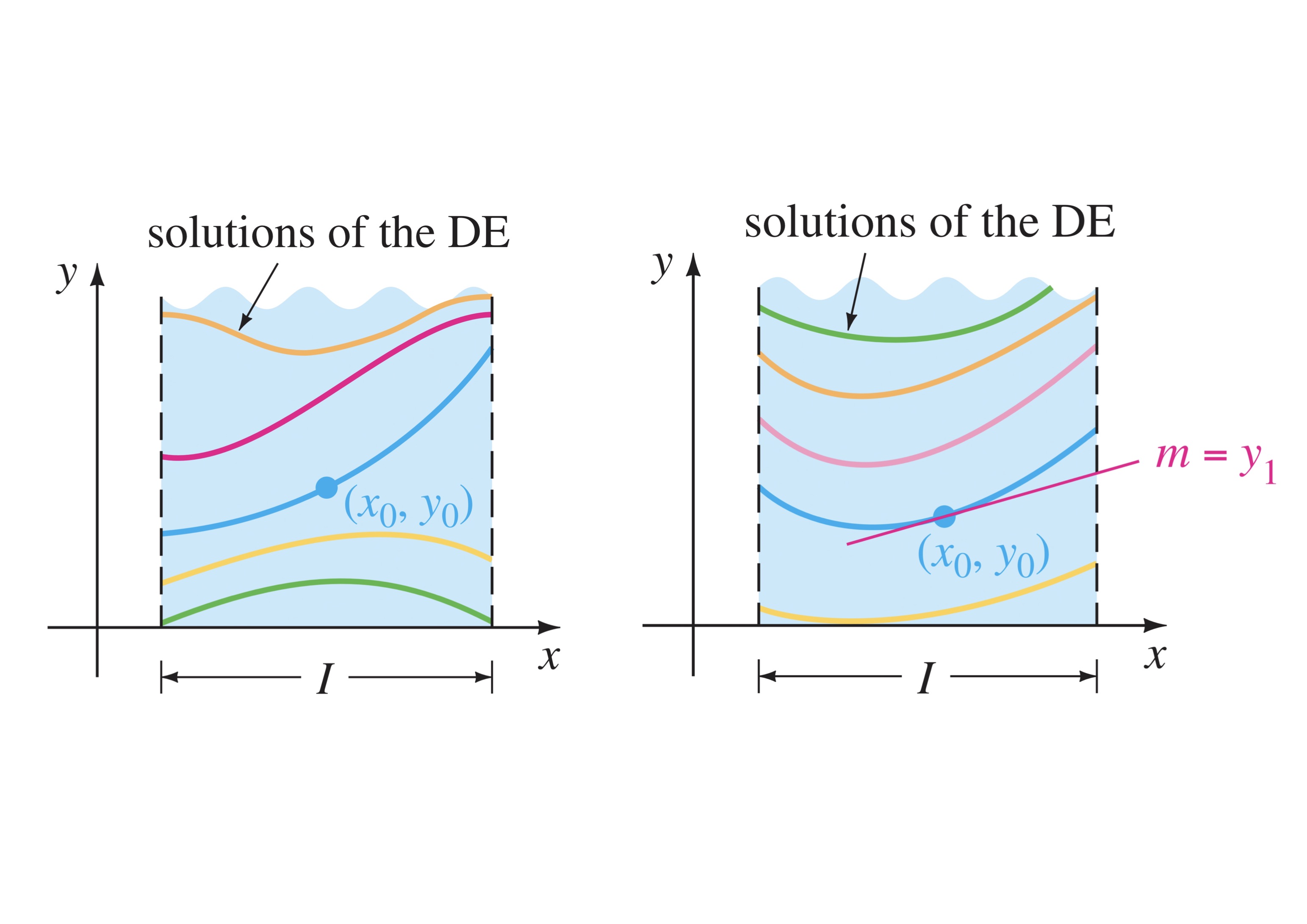
Remark. The words initial conditions derive from physical systems where the independent variable is time \(t\) and where \(y(t_0) = y_0\) and \(y'(t_0) = y_1\) represent the position and velocity, respectively, of an object at some beginning, or initial, time \(t_0\) (See your Mechanics course).

Remark (Initial vs boundary conditions --- a preview). Note that all \(n\) conditions in Equation (2.17) are imposed at the same point \(x_0\) — that is what makes them initial conditions. It is also possible to impose conditions at different points, for example \(y(0)=0\) and \(y(\pi/2)=3\) for a second-order equation. Such conditions are called boundary conditions, and the resulting problem a boundary-value problem (BVP). We will meet BVPs properly when we study second-order equations and their applications; for now, simply register the distinction: initial conditions — one point; boundary conditions — more than one point.

Before the video examples, let us walk one small IVP through in full, so that the two-stage rhythm — general solution first, condition second — is completely explicit. Consider \[\begin{equation*} \dfrac{dy}{dx} = -2y, \quad \text{subject to} \quad y(0)=3. \end{equation*}\] Stage 1 (general solution). The equation is separable. Noting the constant solution \(y=0\) first, then dividing by \(y\) and integrating gives \(\ln|y| = -2x + c\), hence \(y = Ce^{-2x}\) with \(C \in \mathbb{R}\) (the constant solution recovered by \(C=0\), exactly as in Section 2.5.2). Stage 2 (impose the condition). Substituting \(x=0\), \(y=3\): ; \(3 = Ce^{0} = C\). Hence the particular solution is \[\begin{equation*} y = 3e^{-2x}. \end{equation*}\] One family member selected; every other value of \(C\) discarded. Notice how little extra work Stage 2 involved — the substantive effort of an IVP is always the general solution; the initial condition is a final, short act of selection.

Examples

1. \(y'=3y, \quad \text{subject to} \quad y(0)=5.7\)

2. Revisited \(\dfrac{d^3 y}{dx^3}=\sin 2x+e^{-2x}+x^2+x+7, \quad \text{subject to} \quad y(0)=0,y'(0)=1,y''(0)=0\)

Try this for yourself based on the solution we have already obtained previously.

Notice from the above example that:

• We had a third order derivative and we needed three initial conditions in order to find specific values for the three arbitrary constants, i.e. a particular solution. In other words, the order of the differential equation dictates how many initial conditions are required in order to find a particular solution.
• The three conditions here prescribe the value, slope, and concavity of the solution curve at \(x_0=0\) — one condition per constant, all at the same point.
  

3. \(\dfrac{d y}{dx}=-\dfrac{x}{y}, \quad \text{subject to} \quad y(4)=-3\)

Remark (Branches and the interval of definition). Example 3 rewards a second look, because it surfaces two ideas that the earlier examples could not. The general solution is the implicit family \(x^2 + y^2 = c\) (circles — compare the direction field you sketched for this very equation in the exercises of Section 2.4.3). The initial condition gives \(c = 4^2+(-3)^2 = 25\). But making the solution explicit requires choosing a branch: \(y = +\sqrt{25-x^2}\) or \(y = -\sqrt{25-x^2}\). The initial condition decides — since \(y(4) = -3 < 0\), the particular solution is the lower semicircle, \[y = -\sqrt{25-x^2}.\] Moreover, this solution is only defined — as a differentiable function satisfying the DE — on the open interval \((-5, 5)\), which contains \(x_0 = 4\). At \(x = \pm 5\) the curve turns vertical and \(y=0\) makes the equation itself undefined. Two habits to take away: (i) when an implicit family branches, the initial condition selects the branch; (ii) a particular solution always lives on an interval of definition containing \(x_0\), and it is good practice to state it.

4. \((e^{2y}-y) \cos x \dfrac{d y}{dx}=e^y \sin 2x, \quad \text{subject to} \quad y(0)=0\)

Thinking Questions:

1. Clicking a point in the direction field widget imposes an initial condition and traces one curve. What would it mean, geometrically, if an IVP had two different particular solutions? What would the direction field have to look like at \((x_0, y_0)\)?
2. For a first-order equation, suppose you were given two conditions, \(y(0)=1\) and \(y(2)=5\). Is this an initial-value problem? Would you expect a solution to exist at all? (Think about how many arbitrary constants you have to play with.)
3. In Example 2, the three conditions fix \(y\), \(y'\), and \(y''\) at the same point. Could you instead fix \(y\) at three different points and expect to pin down the same three constants? What kind of problem would that be?

Exercise

In the problems below, find an explicit solution for the given initial-value problem. As a challenge, also state the largest interval of definition containing \(x_0\) on which your solution is valid.

1. \(\dfrac{d x}{dt}=4(x^2+1); \quad x(\pi/4)=1\)

2. \(\dfrac{d y}{dx}=\dfrac{y^2-1}{x^2-1}; \quad y(2)=2\)

3. \(x^2\dfrac{d y}{dx}=y-xy; \quad y(-1)=-1\)

Did you get it?

Check your understanding of some of the concepts covered at this stage by attempting the DYGIT? on Initial Value Problems. This is a formative assessment task and does not count for marks so please do it on your own to ascertain your own learning.

2.7 First-Order Models: The Formal Modelling Process

“All models are wrong, but some are useful.” - George E. P. Box (1919-2013)

Everything in this chapter so far has been the solve stage of our cycle. This section returns to formulate — and then, for the first time, we will run the entire cycle end-to-end on real questions: motivate, formulate, solve (with the very methods you have just learned), and interpret. This is the moment the course has been building toward since Chapter 1.

There is no fixed algorithm for constructing a mathematical model that works in all situations — modelling is partly an art. Different people, with different knowledge and different bags of tricks, may build different models of the same system, and for any real system there is no perfect model: one always trades off accuracy, flexibility, and cost. But while there is no algorithm, there is a reliable discipline. We shall follow the ordered sequence of tasks below to build and verify each model in this course, returning to earlier steps whenever a later one exposes a problem:

1. Problem Identification — state precisely what you wish to explore, sharply enough that the verbal description can be translated into mathematical symbols. In real life, nobody hands you the problem; identifying it is itself work.
2. Assumption Specification — you cannot include every factor. Choose which to keep, which to neglect, and which relationships between the kept factors to posit. State these honestly: they are the fine print of every conclusion you will draw.
3. Variable Classification — name your variables, identify which is dependent and which independent, and fix units.
4. Model Construction — translate the assumptions into mathematics: for us, a differential equation, typically with an initial condition.
5. Model Problematization — before solving, interrogate the model’s behaviour: does the sign and size of the rate of change match your experiential and empirical expectations in the obvious special cases? This cheap step catches wrong models early, and you will see it do exactly that below.
6. Model Solution — solve, using the appropriate method for the equation’s classification. Verify your solution.
7. Model Interpretation, Verification, and Validity — say what the solution means, check it answers the original problem, and test it against data where possible. Remember that a model is only ever corroborated by data, never proven: repeated verification under certain conditions does not promote a model to a law.
8. Model Refinement, Implementation, Management, and Maintenance — identify what the model gets wrong or leaves out, and feed that back into a better model. Also: make the model usable and explicable to the people who will rely on it.

Remark. Steps 5 and 7 are where marks are won and lost in this course — and where careers are made in practice. Anyone can be taught to separate variables; the modeller’s real skill is knowing whether the equation deserved solving in the first place, and whether the answer deserves believing.

Conceptual and Mathematical Formulations

A conceptual formulation invariably precedes any mathematical formulation. It can be a graph, a diagram, a rate-flow or compartment picture, or reside “purely in the mind” — and it is expressed in verbal language which must then be translated into formal mathematical statements. The tables below collect the standard translations. Here \(k\) is a positive constant (\(k>0\)), called the constant of proportionality.

Verbal Statement	Mathematical Statement
\(y\) is directly proportional to \(x\)	\(y = kx\)
\(y\) is directly proportional to the \(n\)-th power of \(x\)	\(y = k x^{n}\)
\(y\) is inversely proportional to \(x\)	\(y = \frac{k}{x}\)
\(y\) is inversely proportional to the \(n\)-th power of \(x\)	\(y = \frac{k}{x^{n}}\)
\(y\) is negatively proportional to \(x\)	\(y = - kx\)
\(z\) is proportional to \(x\) and \(y\)	\(z = k x y\)

Question: What does each of these look like graphically?

Similarly, for a dynamic quantity \(x = x(t)\):

Verbal Statement	Mathematical Statement
The value of the dependent variable, \(x\), at any time \(t\)	\(x(t)\)
The rate of change of \(x\) at any time \(t\)	\(\dot x(t)\)
The rate of change of the rate of change of \(x\) at any time \(t\)	\(\ddot x(t)\)

Many physical concepts — velocity, acceleration, growth, decay, cooling — describe change, and hence enter a model as derivatives. A model is therefore very often a differential equation, and the sections that follow build exactly such models.

Figure 3: Some well-known models showing applications of differential equations

Remark (A promise kept). In the Day Zero tutorial you built a symbolic model: “the rate at which the dam level changes depends on inflow minus outflow.” You now own every tool needed to make that sentence mathematics: writing \(V(t)\) for the stored volume, the formulation is \(\frac{dV}{dt} = \text{in}(t) - \text{out}(t)\) — a first-order differential equation, solvable by direct integration whenever the inflow and outflow are known functions of time, with the observed dam level on a given date as the initial condition. Every model in this section is built by exactly this dam-level logic: identify what flows in, what flows out, and write the balance as a rate.

2.8 Models involving Growth

Interest in how populations tend to grow was stimulated in the late eighteenth century when Thomas Malthus (1766–1834) published “An Essay on the Principle of Population as It Affects the Future Improvement of Society”. Malthus put forth an exponential growth model for human population and concluded that the population would eventually exceed the capacity to grow an adequate food supply. Although the assumptions of the Malthusian model leave out factors important to population growth (so the model has proven inaccurate for technologically developed countries), it is instructive to examine it as a basis for later refinement — and it is the perfect entry point into modelling continuous change.

We will build three population models in this section, each one repairing a defect exposed in the previous one. Watch the problematization step do the work each time: the story of this section is not three formulas, but one quality-control test — what does the model say when \(P\) is zero, or at capacity? — applied three times with increasing payoff.

Example 2.1 (Model 1 - A Simple Population Model) Suppose that the world population is increasing at a rate which is proportional to the number of people living at any particular time.

1. Problem Identification Suppose the population is \(P_{0}\) at the time \(t = t_{0}\), and we are interested in predicting the population \(P\) at some future time \(t = t_{1}\). We want to find a population function \(P(t)\) for \(t_{0} \leq t \le t_{1}\) satisfying \(P(t_{0}) = P_{0}\). Symbolically,

\[\begin{equation*} \text{Change in population} \propto \text{Population size}, \end{equation*}\] where \(\propto\) is the mathematical symbol that means “is proportional to”.

2. Assumption Specification Consider some factors that pertain to population growth. Two obvious ones are the birthrate and the death rate. The birthrate is influenced by infant mortality, availability of contraceptives, health care during pregnancy, and so forth; the death rate by sanitation and public health, wars, pollution, medicine, diet, and so forth. Other factors include immigration and emigration, living space restrictions, availability of food and water, and epidemics.

For our first model, let us neglect all of these except birth and death, occurring at fixed per-capita rates — we can revise later if dissatisfied. Assume that during a small time period \(\Delta t\), a fraction \(b\,\Delta t\) of the population is newly born and a fraction \(c\,\Delta t\) dies:

\[\begin{equation*} \text{New population} = \text{Old population}+\text{Number of births}-\text{Number of deaths}, \end{equation*}\] i.e. \[\begin{equation*} P(t + \Delta t) = P(t) + b P(t)\Delta t - c P(t) \Delta t, \end{equation*}\] or \[\begin{equation*} \dfrac{\Delta P}{\Delta t} = b P - c P = (b - c) P. \end{equation*}\]

3. Variable Classification Let \(P\) be the population at time \(t\), so \(P=P(t)\): \(P\) dependent, \(t\) independent.

4. Model Construction Letting \(\Delta t \to 0\), the average rate of change becomes the instantaneous rate \(\frac{dP}{dt}\), and writing \(k=b-c\) with \(b > c\) we obtain: Solve \[\begin{equation} \dfrac{\textrm{d} P}{\textrm{d}t} = k P, \tag{2.20} \end{equation}\] subject to \[\begin{equation*} P(t_{0}) = P_{0}, \end{equation*}\] where \(k>0\) is the growth constant. Equation (2.20) is a first-order linear ordinary differential equation with constant coefficients — classify it yourself and check — and is referred to as the Malthusian model.

5. Model Problematization Before solving, interrogate the model:

• If \(P > 0\), then \(\frac{\textrm{d} P}{\textrm{d}t} > 0\): positive populations grow. Expected.
• What about \(P = 0\)? Then \(\frac{\textrm{d} P}{\textrm{d}t} = 0\): an empty world stays empty — no spontaneous generation. Sensible. (Note that \(P \equiv 0\) is precisely the trivial solution of Section 2.4.1, and there is no need to interrogate \(P<0\): a negative head-count is outside the model’s physical domain.)

Hold onto that \(P=0\) check — it passes here, and its failure will be exactly how we catch Model 2 misbehaving.

6. Model Solution Equation (2.20) is separable (it is also amenable to other methods — thinking question below). Noting the constant solution \(P \equiv 0\) first, then separating for \(P>0\): \[\begin{equation*} \dfrac{ \textrm{d} P}{P} = k \textrm{d} t, \end{equation*}\] and integrating both sides (since populations are positive, \(\ln|P| = \ln P\) here): \[\begin{equation} \tag{2.21} \ln{P} = k t + c. \end{equation}\] Applying the initial condition \(P(t_{0}) = P_{0}\) gives \(c = \ln{P_{0}} - k t_{0}\), and substituting back and simplifying: \[\begin{equation*} \ln{\frac{P}{P_{0}}} = k (t - t_{0}). \end{equation*}\] Exponentiating both sides and multiplying by \(P_0\), we obtain \[\begin{equation} \tag{2.22} P(t) = P_{0} e^{k (t - t_{0})}. \end{equation}\]

Equation (2.22) is the Malthusian model of population growth: the population grows exponentially with time. (And there is Euler’s number, exactly as promised in the Methods section: a quantity whose rate of change is proportional to itself is an exponential, always.)

Thinking Question: Is separation of variables the only method of solution for Equation (2.20)?

7. Model Interpretation, Verification, and Validity The Malthusian model (2.20) can also be solved computationally for ranging values of the growth constant \(k=0;0.5;1;1.5;2\):

• The blue line represents \(k=0\): the population remains constant in the absence of net growth.
• The orange, green, red, and purple lines represent \(k>0\): the population grows exponentially, at a rate governed by \(k\).

Let us now test the model against real data — our own. According to Statistics South Africa’s mid-year estimates, South Africa’s population was approximately \(59{,}62\) million in 2020 and \(63{,}02\) million in 2024. Taking \(t_0 = 2020\) and fitting the growth constant from these two data points: \[\begin{equation*} k = \frac{1}{4}\ln\!\left(\frac{63{,}02}{59{,}62}\right) \approx 0{,}0139 \text{ per year}, \end{equation*}\] that is, roughly \(1{,}4\%\) per year — pleasingly close to Stats SA’s own reported year-on-year growth rate of about \(1{,}3\%\). The fitted model then predicts approximately \(68{,}5\) million in 2030, \(73{,}4\) million in 2035, and \(90{,}4\) million by 2050, with a doubling time of \(\ln 2 / k \approx 50\) years.

Should we believe these predictions? The near ones, cautiously; the far ones, no. The model assumes \(k\) is constant forever, but South Africa’s growth rate — like most countries’ — has been declining for decades as birth rates fall. A constant-\(k\) extrapolation therefore overshoots further and further the deeper into the future it reaches. This is Malthus’s own error, and it is worth naming precisely: the model is not wrong because the mathematics is wrong; it is wrong because an assumption (constant per-capita growth) fails over long horizons. Interpretation means knowing the difference.

8. Model Refinement, Implementation, Management, and Maintenance Exponential growth continues without bound — no environment supports that indefinitely. Real populations face limited food, water, and space. The refinement: build the limit into the model. This is Model 2.

Example 2.2 (Model 2 - Refining the Model to incorporate a Carrying Capacity) Suppose now that the population increases at a rate which is proportional to the difference between the current population size and the maximum possible size the population could attain.

1. Problem Identification As before, we seek \(P(t)\) with \(P(t_0)=P_0\). Symbolically, the problem can be identified either as \[\begin{equation*} \text{Change in population} \propto (\text{Current population size} - \text{Carrying capacity}), \end{equation*}\] or \[\begin{equation*} \text{Change in population} \propto (\text{Carrying capacity}-\text{Current population size}). \end{equation*}\]

2. Assumption Specification We consider the same assumptions as in Model 2.1, now with one addition: the environment supports at most a fixed maximum population.

3. Variable Classification Again let \(P=P(t)\), and let \(M\) be the maximum possible size of the population, known as the carrying capacity.

4. Model Construction Our verbal statement translates into two candidate models: \[\begin{equation} \dfrac{\textrm{d} P}{\textrm{d}t} = k(P-M), \tag{2.23} \end{equation}\] or \[\begin{equation} \dfrac{\textrm{d} P}{\textrm{d}t} = k(M-P), \tag{2.24} \end{equation}\] where \(k > 0\). Which is the correct formulation? Pause here and see if you can determine this for yourself.

5. Model Problematization This is problematization earning its keep: the mathematics alone cannot choose between (2.23) and (2.24) — only expected behaviour can.

Case \(M > P\) (room to grow; expect \(\frac{dP}{dt}>0\)):

• Equation (2.23): \(P-M <0\) and \(k>0\) give \(\frac{\textrm{d} P}{\textrm{d}t} < 0\). Populations below capacity would shrink. Reject.
• Equation (2.24): \(M-P >0\) gives \(\frac{\textrm{d} P}{\textrm{d}t} > 0\). Sensible.

Case \(M < P\) (over capacity; expect decline, \(\frac{dP}{dt}<0\)):

• Equation (2.23): \(P-M >0\) gives \(\frac{\textrm{d} P}{\textrm{d}t} > 0\): overcrowding would accelerate growth. Reject.
• Equation (2.24): \(M-P <0\) gives \(\frac{\textrm{d} P}{\textrm{d}t} < 0\). Sensible.

So we choose Equation (2.24): Solve \[\begin{equation} \dfrac{\textrm{d} P}{\textrm{d}t} = k(M-P), \tag{2.25} \end{equation}\] subject to \(P(t_{0}) = P_{0}\), with \(k>0\).

6. Model Solution The equation is separable. Note first the constant solution: \(P \equiv M\) makes both sides zero — a population exactly at capacity stays there. For \(P \neq M\), separate: \[\begin{equation*} \dfrac{ \textrm{d} P}{M-P} = k \textrm{d} t, \end{equation*}\] and integrate: \[\begin{equation*} -\ln{|M-P|} = k t + c \quad\Longrightarrow\quad \ln{|M-P|} = -k t + c. \end{equation*}\] Exponentiating and absorbing \(\pm e^{c}\) into a constant \(A\) (the absorb-and-recover pattern of Section 2.5.2 — and note \(A=0\) recovers the constant solution \(P=M\)): \[\begin{equation*} M-P = Ae^{-k t}, \end{equation*}\] giving the general solution \[\begin{equation*} P(t) = M-Ae^{-k t}. \tag{2.26} \end{equation*}\] Applying \(P(t_{0}) = P_{0}\) gives \(A = (M-P_{0})e^{k t_{0}}\), and hence \[\begin{equation} P(t) = M-(M-P_{0}) e^{-k (t-t_{0})}. \tag{2.27} \end{equation}\]

Thinking Question: Is the above the only method of solution for Equation (2.25)?

7. Model Interpretation, Verification, and Validity Solving computationally for \(P_0=100\), \(k=5\), and carrying capacities \(M=50;100;150;200\):

• The orange line (\(M=P_0=100\)): the population remains constant — the constant solution \(P=M\) visible in the flesh.
• The red and green lines (\(M=200, 150\)): growth toward capacity, stabilizing as it arrives — no longer unbounded exponential growth.
• The blue line (\(M=50\)): a population above capacity decays down to it.

As \(t \to \infty\), Equation (2.27) gives \(P \to M\) from either side: every solution is funnelled to the carrying capacity. (You have seen this funnelling picture before — it is exactly the direction-field behaviour of \(y' = 1-y\) from Tutorial 2, with the flat line at the capacity.)

But now apply our quality-control test: what does the model say at \(P=0\)? From (2.25), \(\frac{\textrm{d} P}{\textrm{d}t}\big|_{P=0} = kM > 0\). An empty world spontaneously generates people — and at the model’s fastest rate! Worse, the growth rate \(k(M-P)\) is largest when the population is smallest, which inverts all biological sense: two organisms cannot out-reproduce two million. The model has the right destination (\(M\)) but the wrong engine.

8. Model Refinement, Implementation, Management, and Maintenance The fix must make the growth rate small when \(P\) is small (few individuals to reproduce) and small when \(P\) nears \(M\) (competition for resources) — so the rate should be proportional to both \(P\) and \((M-P)\) at once. That is Model 3.

Example 2.3 (Model 3 - Refining the Model to Reflect Limited Growth) Suppose now that the population increases at a rate which is proportional to the current population size and the difference between the current population size and the maximum possible size the population could attain.

1. Problem Identification As before, with the refined verbal statement translating to either \[\begin{equation*} \text{Change in population} \propto [\text{Current population} \times (\text{Current population} - \text{Carrying capacity})], \end{equation*}\] or \[\begin{equation*} \text{Change in population} \propto [\text{Current population} \times (\text{Carrying capacity}-\text{Current population})]. \end{equation*}\]

2–3. Assumptions and Variables as in Model 2.2.

4. Model Construction The two candidates: \[\begin{equation} \dfrac{\textrm{d} P}{\textrm{d}t} = kP(P-M), \tag{2.28} \end{equation}\] or \[\begin{equation} \dfrac{\textrm{d} P}{\textrm{d}t} = kP(M-P). \tag{2.29} \end{equation}\]

5. Model Problematization Run the same sign analysis as in Model 2.2 to choose — do this yourself before reading on. You should reject (2.28) and select (2.29): Solve \[\begin{equation} \dfrac{\textrm{d} P}{\textrm{d}t} = kP(M-P), \tag{2.30} \end{equation}\] subject to \(P(t_{0}) = P_{0}\), with \(k>0\). And now re-run the quality-control test that caught Model 2: at \(P=0\), the rate is \(k\cdot 0\cdot M = 0\) — an empty world stays empty. At \(P=M\), the rate is zero — capacity is an equilibrium. Both constant solutions, \(P\equiv 0\) and \(P\equiv M\), sit inside the model, and small populations grow slowly, as biology demands. The defect is repaired.

This model was first introduced by the Dutch mathematical biologist Pierre-Francois Verhulst (1804–1849), who read Malthus’s essay and extended the model for populations with resource limitations. Equation (2.30) is the logistic growth model, and it agrees well with populations of organisms with simple life histories — for instance yeast growing in a culture where space is limited. It is also the very equation \(y' = y(1-y)\) (there with \(k=M=1\)) that you explored in the direction field widget in Section 2.4.3: you have already seen everything we are about to derive.

6. Model Solution The equation is separable, and this time both constant solutions \(P\equiv 0\), \(P\equiv M\) are noted before dividing. For \(0 < P < M\): \[\begin{equation*} \dfrac{ \textrm{d} P}{P(M-P)} = k \textrm{d} t. \end{equation*}\] Partial fraction decomposition (dust off your Mathematics notes) gives \[\begin{equation*} \dfrac{1}{P (M - P)} = \dfrac{1}{M} \left(\dfrac{1}{P} + \dfrac{1}{M - P}\right), \tag{2.31} \end{equation*}\] so that, multiplying through by \(M\), the separated equation becomes \[\begin{equation*} \left(\dfrac{1}{P} + \dfrac{1}{M - P}\right) \textrm{d} P = k M\, \textrm{d} t. \end{equation*}\] Integrating both sides: \[\begin{equation} \ln{P} - \ln{(M - P)} = k M t + c, \tag{2.32} \end{equation}\] for some arbitrary constant \(c\) (with \(0<P<M\), both logarithms need no absolute values). Using the initial condition to evaluate \(c\): \[\begin{equation*} c = \ln{\dfrac{P_{0}}{M - P_{0}}} - k M t_{0}. \end{equation*}\] Substituting into (2.32) and simplifying: \[\begin{equation*} \ln{\dfrac{P (M - P_{0})}{P_{0}(M - P)}} = k M(t - t_{0}). \end{equation*}\] Exponentiating and solving for \(P\) (a few lines of algebra — do them): \[\begin{equation} P(t) = \dfrac{P_{0} M e^{k M (t - t_{0})}} {M - P_{0} + P_{0} e ^{k M (t - t_{0})}}. \tag{2.33} \end{equation}\]

7. Model Interpretation, Verification, and Validity Solving computationally:

The s-shaped (sigmoid) curve is called a logistic curve.

To read off the long-run behaviour, divide numerator and denominator of (2.33) by \(e^{kM(t-t_0)}\): \[\begin{equation} P(t) = \frac{M P_{0}}{P_{0} + (M - P_{0}) e^{-k M (t - t_{0})}}. \tag{2.34} \end{equation}\] As \(t \to \infty\) the exponential term vanishes, and \(P(t) \to \dfrac{MP_0}{P_0} = M\): every positive starting population is carried to the capacity. Moreover, differentiating Equation (2.30) itself (chain rule on the right): \[\begin{equation*} P'' = k M P' - 2 k P P' = k P' (M - 2 P), \end{equation*}\] so \(P'' = 0\) when \(P = \frac{M}{2}\): the population grows fastest at exactly half the carrying capacity, after which growth diminishes toward zero. This has a practical use: if data suggests a population’s growth has just peaked, then the current population is an estimate of \(\frac{M}{2}\) — doubling it estimates the carrying capacity itself.

Thinking Questions:

• What do the above graphs tell us? Why are the two plots vastly different? (Hint: look at the code for both. What differs?)
• What happens to the population as \(t \to \infty\) if \(P_0 > M\)? Does Equation (2.34) still deliver it to \(M\)? From above or below?
• If in 1970 \(P = 4 \times 10^9\), in 1990 \(P = 5 \times 10^9\) and \(M = 12 \times 10^9\), estimate the world population in 2011.

8. Model Refinement, Implementation, Management, and Maintenance

Thinking Question: Can you think of ways in which we could refine Model 2.3 further? (Seasonal birth rates? Harvesting or emigration at a constant rate? A capacity \(M\) that itself changes with technology — what would that do to the equation?)

Explore: the population playground

Reading about these three models is one thing; feeling how their parameters shape the future is another. The widget below plots the exact solution of whichever model you choose. Drag the sliders and watch the curve respond; press Freeze curve to pin the current curve in grey for comparison before changing a slider.

Model: 1: Malthus   dP/dt = kP 2: Carrying capacity   dP/dt = k(M − P) 3: Logistic   dP/dt = kP(M − P)

P₀ 20 k 0.30 M 200

Try this with the widget:

1. On Model 1, freeze a curve, then double \(k\). Compare the two curves at the right-hand edge. Now halve \(P_0\) instead — which parameter matters more for the long run, the starting size or the growth rate?
2. On Model 2, drag \(P_0\) close to \(0\) and watch the initial slope of the curve. This is the “empty world grows fastest” defect from the problematization step — visible with your own eyes.
3. On Model 3, place \(P_0\) well below \(M/2\) and find the green dot: the moment of fastest growth, at exactly \(P = M/2\). Then set \(P_0\) above \(M\), and \(P_0 = M\) exactly. Relate all three behaviours to the constant solutions and the direction field of \(y'=y(1-y)\) from Section 2.4.3.
4. Set the three models up with the same \(P_0\), \(k\)-slider value, and \(M\), freezing each in turn. For small \(t\) the three curves nearly agree — why? (Think about what \(k(M-P)\) and \(kP(M-P)\) look like when \(P\) is far from both \(0\) and \(M\).)

Did you get it?

Check your understanding of some of the concepts covered at this stage by attempting the DYGIT? on Growth Models. (Link to be added once the quiz is created on Moodle.)