Chapter 3 Second-Order Differential Equations and Oscillatory Models

“The same equations have the same solutions.” - Richard Feynman, The Feynman Lectures on Physics, Vol. II, §12–1

In Chapter 1 we laid the course out as three acts. Act I is now complete. Growth, decay, cooling, drug elimination: every model we built rested on a single idea — the rate at which a quantity changes depends on how much of it there is. That idea took us a long way, from rhino reserves to the age of a fossil.

But look around, and a great deal of the world does something none of those models can do. A car rocks after it goes over a speed bump. A guitar string hums. A pendulum swings. The voltage in the circuit charging your phone rises and falls fifty times a second. Tall buildings sway in the wind. Things oscillate — and Act I cannot describe a single one of them.

Act II begins here.

Why Act I cannot oscillate

This is worth understanding properly, because it tells us exactly what is missing.

Every Act I model had the form \(\frac{dy}{dt} = f(y)\): the rate depended only on the current value of \(y\). Suppose a solution of such a model were to oscillate. Then at the top of each swing it would have to turn around, and at that instant \(\frac{dy}{dt} = 0\). But \(\frac{dy}{dt} = f(y)\), so \(f(y) = 0\) there — which means the solution is sitting exactly on an equilibrium. And an equilibrium is itself a solution curve: a flat line. Since solution curves of a well-behaved equation cannot cross (Section 2.4.3), our solution cannot leave that line. It is stuck. It never turns around at all.

So a model of this kind can rise, fall, or level off — but it can never turn back. That is why every solution we met in Act I was monotone: growing, decaying, or settling towards a limit.

What is missing is memory. To swing past the middle and keep going, a pendulum has to “know” which way it is currently moving. Its position alone is not enough; the model needs its velocity as well. And the moment velocity enters the model, so does its rate of change — acceleration, a second derivative.

Remark. A careful reader may object that \(\frac{dy}{dx} = \cos x\) is first order and has the oscillating solution \(y = \sin x + c\). True — but there the rate depends on \(x\), not on \(y\). The oscillation has been written into the equation by hand, through the \(\cos x\); nothing in the physics produces it. The claim above is about models in which the system’s own state drives its change, which is what every Act I model did.

Where second derivatives come from: Newton’s second law

The single most important source of second-order equations in science is Newton’s second law of motion, \[ \text{Force} = \text{mass} \times \text{acceleration}. \] If \(x(t)\) is the position of an object at time \(t\), then its velocity is \(\dot{x}\) and its acceleration is \(\ddot{x}\). So Newton’s law reads \(F = m\ddot{x}\) — and as soon as we say what the forces are, we have a second-order differential equation.

Let us build the central model of this chapter, using the modelling process from Section 2.7. A mass \(m\) is attached to a spring and slides on a surface. Let \(x(t)\) be its displacement from the resting position, positive to the right. Two forces act on it:

• The spring. Pull the mass to the right and the spring pulls it back to the left; push it left and the spring pushes it right. For a spring that is not stretched too far, this restoring force is proportional to the displacement (Hooke’s law): \(F_{\text{spring}} = -kx\), where the spring constant \(k > 0\) measures its stiffness.
• Friction. Friction always opposes motion, and for many systems it is proportional to the speed: \(F_{\text{friction}} = -b\dot{x}\), where the damping constant \(b \geq 0\).

Newton’s second law then gives \(m\ddot{x} = -kx - b\dot{x}\), or \[\begin{equation} m\ddot{x} + b\dot{x} + kx = 0. \tag{3.1} \end{equation}\]

Problematize before going further. Do the signs make sense? If the mass is to the right (\(x > 0\)), the spring term \(-kx\) is negative: it pulls left, back towards rest. If the mass is moving right (\(\dot{x} > 0\)), the friction term \(-b\dot{x}\) is negative: it resists the motion. And if \(x = 0\) and \(\dot{x} = 0\), then \(\ddot{x} = 0\): a mass at rest in the middle stays there. Every check passes.

Notice what Equation (3.1) is, in the language of Section 2.3: second order, linear, homogeneous, with constant coefficients. That classification is exactly what will tell us how to solve it.

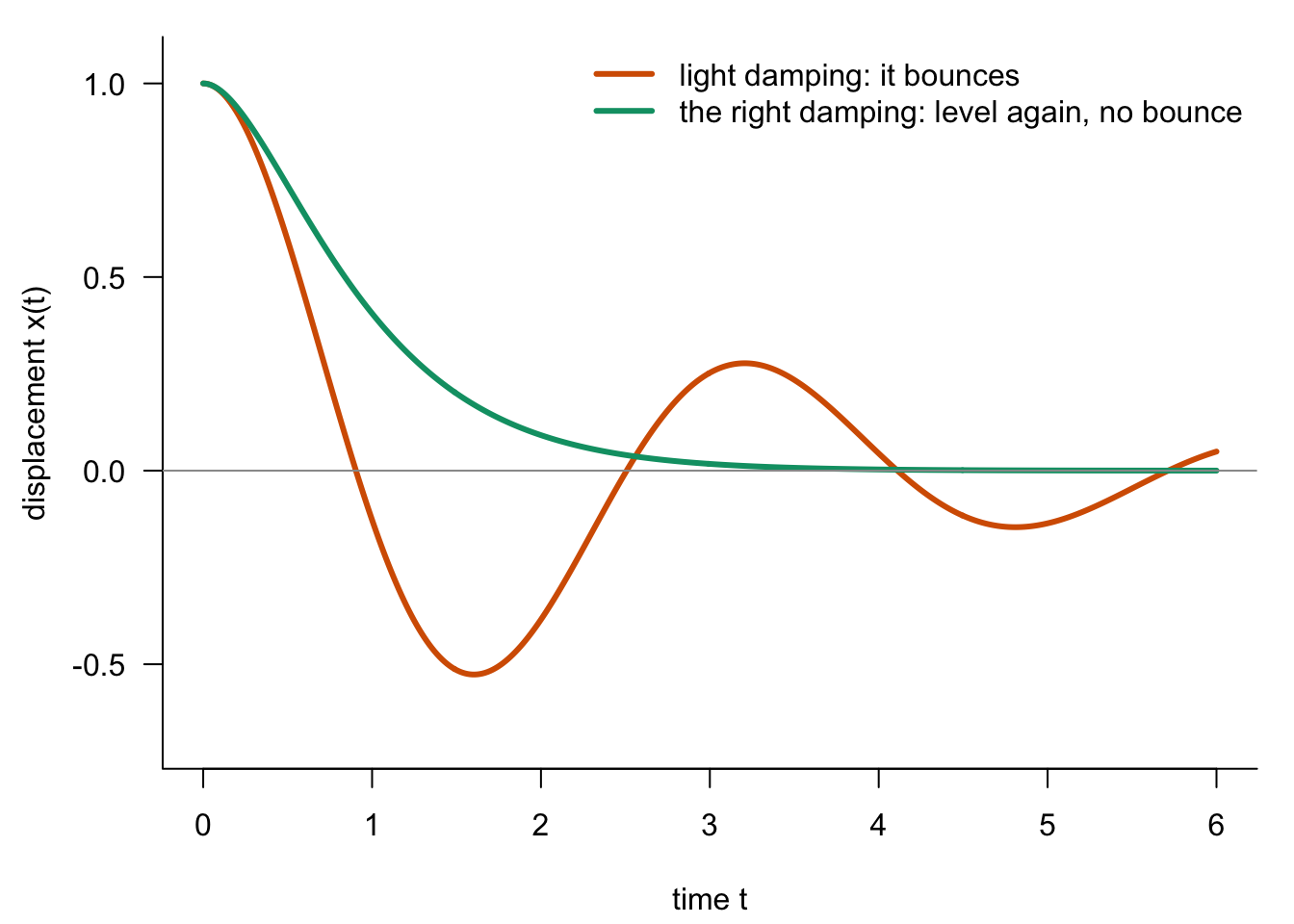
Figure 3.1: The same equation, two amounts of friction: how a car’s body moves after going over a bump. With light damping it bounces; with the right amount of damping it returns to level without bouncing at all.

The same equation, somewhere else entirely

Now for the reason this chapter is worth so much. Consider an electrical circuit containing an inductor (inductance \(L\)), a resistor (resistance \(R\)) and a capacitor (capacitance \(C\)), driven by a voltage source \(E(t)\) — an RLC circuit, of the kind inside every radio, charger and speaker. Kirchhoff’s voltage law gives, for the charge \(q(t)\) on the capacitor, \[\begin{equation} L\ddot{q} + R\dot{q} + \frac{1}{C}\,q = E(t). \tag{3.2} \end{equation}\]

Set the two equations side by side:

Mass on a spring		RLC circuit
displacement \(x\)	\(\longleftrightarrow\)	charge \(q\)
mass \(m\)	\(\longleftrightarrow\)	inductance \(L\)
friction \(b\)	\(\longleftrightarrow\)	resistance \(R\)
spring stiffness \(k\)	\(\longleftrightarrow\)	\(1/C\)
applied force \(F(t)\)	\(\longleftrightarrow\)	applied voltage \(E(t)\)

They are the same equation with the letters changed. A mass bouncing on a spring and the charge sloshing around a circuit have nothing physical in common — one is mechanics, the other electromagnetism — and yet the mathematics cannot tell them apart. Solve one, and you have solved the other. That is the meaning of the quotation at the head of this chapter, and it is the deepest reason to learn to solve differential equations at all: you are not learning to solve one problem, you are learning to solve every problem that shares its equation.

The plan for this chapter

Equations (3.1) and (3.2) differ in one important way. The spring-mass system above is left to itself: nothing pushes it once it is released, and its equation is homogeneous. The circuit is driven by the voltage \(E(t)\), so its equation is non-homogeneous. That distinction organises the whole chapter — and it turns out to have a lovely physical meaning:

• The homogeneous equation describes the system’s own natural behaviour when left alone — how it rings, sways or settles by itself.
• The non-homogeneous equation adds the system’s response to being pushed from outside.

We tackle them in that order:

1. Section 3.1 — the homogeneous equation. We learn to solve \(a\ddot{y} + b\dot{y} + cy = 0\), and discover that its behaviour falls into exactly three cases — which will turn out to be the difference between a car that bounces and one that does not.
2. Section 3.2 — the non-homogeneous equation. We learn to find the response to a driving force, by the method of undetermined coefficients.
3. Oscillatory models. We return to the mass on a spring and the RLC circuit with both tools in hand, and use them to predict and interpret free, damped and driven motion.

Learning outcomes

By the end of this chapter, you should be able to:

• Explain why oscillating systems require second-order models, and derive a second-order model from Newton’s second law.
• Solve second-order linear homogeneous equations with constant coefficients, identifying from the discriminant which of the three cases applies.
• Find particular integrals of non-homogeneous equations using the method of undetermined coefficients, including when an adjustment for duplication is required.
• Solve second-order initial value problems, using two initial conditions to determine two arbitrary constants.
• Formulate, solve and interpret models of oscillating systems, including a mass on a spring and an electrical RLC circuit, and recognise when two different physical systems share the same mathematics.

What carries over, and what you will need

Almost everything from Act I comes with us. You will still classify before choosing a method (Section 2.3); still verify a solution by substitution; still solve initial value problems in the order general solution first, conditions second — except that a second-order problem now needs two conditions to fix its two arbitrary constants (Section 2.6). And the modelling habits — formulate, problematize, solve, interpret — apply exactly as before.

Remark (Before you start: check your calculus and algebra). This chapter asks more of your first-year mathematics than anything before it. Experience shows that when students struggle here, it is rarely with the differential equations themselves — it is with the calculus and algebra underneath them. You will need to be fluent with:

• solving quadratic equations, including those with complex roots;
• complex numbers, and Euler’s identity \(e^{i\theta} = \cos\theta + i\sin\theta\);
• differentiating products and compositions (the product and chain rules), since every trial solution will be differentiated twice.

If any of these feel uncertain, revisit them now, using the Prerequisites chapter and your MATH1036A notes. Half an hour spent here will save you far more later in the chapter.

We begin with the simplest case: a system left entirely to itself, described by a homogeneous equation like (3.1). Our first task is to learn how to solve it.

3.1 The Method of Undetermined Coefficients

Every method you have met so far has worked by isolating something. Direct integration needs the derivative alone on one side. Separation of variables needs the variables apart on either side. Now consider

\[ y'' + 3y' + 2y = 0. \]

It is second order, so separation is unavailable. It has \(y\) and its derivatives mixed together on one side, so direct integration is unavailable. None of our tools apply — and yet it has exactly the shape of the spring-mass equation (3.1) from the chapter introduction. We need a new method.

The method we develop here works in two stages, and it is worth knowing the plan before we start:

1. This section: solve the homogeneous equation (right-hand side zero). Its general solution is called the complementary function.
2. The next section: find one solution of the non-homogeneous equation, called the particular integral, by making an educated guess with coefficients to be determined — the “undetermined coefficients” that give the method its name.

The general solution is then the sum of the two. We begin by recalling what homogeneous means.

Definition 3.1 (Homogeneity of a Linear Ordinary Differential Equation) A linear \(n\)th-order differential equation of the form \[\begin{equation} a_{n}(x)\dfrac{d^n y}{dx^n}+a_{n-1}(x)\dfrac{d^{n-1} y}{dx^{n-1}}+\dots+a_{1}(x)\dfrac{d y}{dx}+a_{0}(x)y=0 \tag{3.3} \end{equation}\] is said to be homogeneous, whereas an equation \[\begin{equation} a_{n}(x)\dfrac{d^n y}{dx^n}+a_{n-1}(x)\dfrac{d^{n-1} y}{dx^{n-1}}+\dots+a_{1}(x)\dfrac{d y}{dx}+a_{0}(x)y=g(x) \tag{3.4} \end{equation}\] with \(g(x)\) not identically zero, is said to be non-homogeneous.

For example, \(2y''+3y'-5y=0\) is a homogeneous linear second-order equation, whereas \(x^3 y'''+6y'+10y=e^x\) is a non-homogeneous linear third-order equation.

The general solution of Equation (3.3) must contain \(n\) arbitrary constants — one per order, as we saw with direct integration. Supplying \(n\) conditions at a single point makes it an initial value problem (Section 2.6); supplying conditions at more than one point makes it a boundary value problem.

We now focus on second-order linear equations with constant coefficients, in standard form \[\begin{equation} a y'' + b y' + c y = g(x), \tag{3.5} \end{equation}\] where \(y=y(x)\), the coefficients \(a\), \(b\), \(c\) are constants with \(a \neq 0\), and \(g(x)\) is not identically zero. Its associated homogeneous equation is \[\begin{equation} a y'' + b y' + c y = 0. \tag{3.6} \end{equation}\]

Definition 3.2 (Complementary Function) The general solution of the homogeneous equation (3.6) is called the complementary function of the non-homogeneous equation (3.5), and is denoted \(y_{c}\).

Definition 3.3 (Particular Integral) Any single solution of the non-homogeneous equation (3.5), free of arbitrary constants, is called a particular integral of that equation, and is denoted \(y_{p}\).

Definition 3.4 (General Solution of a Linear Ordinary Differential Equation) The general solution of the non-homogeneous linear equation (3.4) is \[\begin{equation*} y = y_{c} + y_{p}, \end{equation*}\] where \(y_{c}\) is the complementary function (the general solution of the associated homogeneous equation (3.3)) and \(y_{p}\) is any particular integral.

All \(n\) arbitrary constants live in \(y_c\). The particular integral contributes none.

Remark. The complementary function is not a solution of the non-homogeneous equation — substitute it in and you get zero on the left, not \(g(x)\). It is a component which, added to a particular integral, produces the general solution. The particular integral, by contrast, is always a solution of the non-homogeneous equation.

3.1.1 Homogeneous Linear Equations with Constant Coefficients

The first-order case

Start with the simplest possible version: \[\begin{equation*} \dfrac{dy}{dx} - ay = 0, \end{equation*}\] where \(a\) is a constant. This is separable (Section 2.5.2): \[\begin{equation*} \int \frac{dy}{y} = \int a\,dx \quad\Longrightarrow\quad \ln|y| = ax + c_1 \quad\Longrightarrow\quad y = c_2e^{ax}. \end{equation*}\] The solution is an exponential, and the constant \(a\) from the equation has become the rate in the exponent. That is not a coincidence, and it is the key to everything that follows.

Let us consider a few examples:

Why an exponential?

Look at the second-order equation (3.6) and ask what kind of function could possibly satisfy it. We need \(a y'' + b y' + cy\) to add up to exactly zero, for every \(x\). That can only happen if \(y\), \(y'\) and \(y''\) are all the same kind of function — otherwise there is nothing for them to cancel against. A polynomial will not do (differentiating lowers the degree); \(\ln x\) will not do (its derivatives are powers of \(x\)). We need a function whose derivatives are multiples of itself.

You already know such a function. In the Methods section we found that \(e^x\) is its own derivative, and more generally \[\begin{equation*} \dfrac{d}{dx}e^{\lambda x} = \lambda e^{\lambda x}, \qquad \dfrac{d^2}{dx^2}e^{\lambda x} = \lambda^2 e^{\lambda x}. \end{equation*}\] So every derivative of \(e^{\lambda x}\) is just \(e^{\lambda x}\) multiplied by a number. That is precisely what we need.

The auxiliary equation

Take as a trial solution \(y = Ae^{\lambda x}\), where \(A\) is an arbitrary constant and \(\lambda\) is a constant to be found. Then \[\begin{equation*} y = Ae^{\lambda x}, \qquad y' = \lambda Ae^{\lambda x}, \qquad y'' = \lambda^2 Ae^{\lambda x}. \end{equation*}\] Substituting into (3.6): \[\begin{equation*} a\lambda^2 Ae^{\lambda x} + b\lambda Ae^{\lambda x} + cAe^{\lambda x} = 0 \quad\Longrightarrow\quad Ae^{\lambda x}\left(a\lambda^2 + b\lambda + c\right) = 0. \end{equation*}\] Now \(e^{\lambda x}\) is never zero, and \(A \neq 0\) (otherwise we have only the trivial solution). So the bracket must vanish: \[\begin{equation} a \lambda^{2} + b \lambda + c = 0. \tag{3.7} \end{equation}\] This is called the auxiliary equation (or characteristic equation) of (3.6).

Remark (The whole trick, in one sentence). A differential equation has become an algebraic equation. Every derivative turned into a power of \(\lambda\) — \(y''\) became \(\lambda^2\), \(y'\) became \(\lambda\), \(y\) became \(1\) — so solving a differential equation has been reduced to solving a quadratic. That is why this method is so powerful, and why you can read the auxiliary equation straight off the differential equation by inspection: just copy the coefficients.

By the quadratic formula, the roots of (3.7) are \[\begin{equation*} \lambda_{1} = \dfrac{-b - \sqrt{b^{2} - 4 a c}}{2a} \quad \text{and} \quad \lambda_{2} = \dfrac{-b + \sqrt{b^{2} - 4 a c}}{2a}. \end{equation*}\] What kind of roots we get — and therefore what kind of solution — is decided entirely by the discriminant \(b^2 - 4ac\). There are three possibilities, and we examine each in turn.

Two tools we need first

Definition 3.5 (Superposition Principle) Suppose \(y_{1}, y_{2}, \dots, y_{n}\) are solutions of the linear homogeneous equation (3.3). Then any linear combination \[\begin{equation*} y = k_{1}y_{1} + k_{2}y_{2} + \dots + k_{n}y_{n} = \sum_{i=1}^{n} k_{i}y_{i}, \end{equation*}\] where the \(k_{i}\) are arbitrary constants, is also a solution.

Superposition only works because the equation is linear and homogeneous: substitute a sum of solutions into the left-hand side, and linearity splits it into a sum of left-hand sides, each of which is zero. Neither property can be dropped — it fails for nonlinear equations, and it fails for non-homogeneous ones (two solutions of \(y' = 1\) do not sum to a solution).

Definition 3.6 (Linearly Dependent and Independent Functions) Two functions \(f(x)\) and \(g(x)\) are linearly dependent on an interval \(I\) if there exist constants \(k_1\) and \(k_2\), not both zero, such that \[\begin{equation*} k_1 f(x) + k_2 g(x) = 0 \quad \text{for every } x \in I. \end{equation*}\] Otherwise they are linearly independent. In practice, for two nonzero functions: they are linearly dependent exactly when one is a constant multiple of the other.

Why do we care? A second-order equation needs two genuinely different solutions to make a general solution with two arbitrary constants. If our two solutions were multiples of each other — say \(e^{2x}\) and \(5e^{2x}\) — then \(k_1e^{2x} + k_2(5e^{2x}) = (k_1 + 5k_2)e^{2x}\) collapses to a single constant, and we have not really found two solutions at all. Linear independence is the test that stops this happening.

Case 1: Distinct real roots, \(b^{2} - 4 a c > 0\)

The auxiliary equation has two different real roots \(\lambda_1 \neq \lambda_2\), giving two solutions \[\begin{equation*} y_{1}(x) = e^{\lambda_{1} x} \quad \text{and} \quad y_{2}(x) = e^{\lambda_{2} x}. \end{equation*}\] These are linearly independent, since their ratio \(e^{(\lambda_1 - \lambda_2)x}\) is not constant. The differential equation (3.6) is linear and homogeneous, so by superposition the general solution is \[\begin{equation*} y(x) = c_{1} e^{\lambda_{1} x} + c_{2} e^{\lambda_{2} x}, \end{equation*}\] with two arbitrary constants \(c_{1}\) and \(c_{2}\) — exactly as many as the order demands.

Example

Solve \(\ddot{x} + 3 \dot{x} + 2 x = 0\), subject to \(x(0) = 0\) and \(\dot{x}(0) = 1\).

With trial solution \(x(t) = Ae^{\lambda t}\), the auxiliary equation is \[\begin{equation*} \lambda^{2} + 3 \lambda + 2 = 0 \quad\Longrightarrow\quad (\lambda+1)(\lambda+2) = 0, \end{equation*}\] with roots \(\lambda_{1} = -1\) and \(\lambda_{2} = -2\). The general solution is \[\begin{equation*} x(t) = c_{1} e^{-t} + c_{2} e^{-2t}. \end{equation*}\] Now apply the initial conditions — general solution first, conditions second. Since \(\dot{x}(t) = -c_1e^{-t} - 2c_2e^{-2t}\): \[\begin{align*} x(0) = 0 &\quad\Longrightarrow\quad c_1 + c_2 = 0, \\ \dot{x}(0) = 1 &\quad\Longrightarrow\quad -c_1 - 2c_2 = 1. \end{align*}\] Solving simultaneously gives \(c_1 = 1\) and \(c_2 = -1\), so \[\begin{equation*} x(t) = e^{-t} - e^{-2t}. \end{equation*}\]

Notice that a second-order problem needed two initial conditions to fix two constants, exactly as the IVP section predicted.

Case 2: A repeated real root, \(b^{2} - 4 a c = 0\)

Now the two roots coincide, \(\lambda_{1} = \lambda_{2} = \lambda = -\dfrac{b}{2a}\), and we get only one solution, \[\begin{equation*} y_{1}(x) = e^{\lambda x}. \end{equation*}\] But a second-order equation needs two linearly independent solutions, so there must be a second one somewhere. We cannot use \(e^{\lambda x}\) again — that is linearly dependent on \(y_1\). So we try something similar to, but independent of, the first: multiply by the independent variable, \(y = xe^{\lambda x}\).

Then \(y' = e^{\lambda x} + \lambda xe^{\lambda x}\) and \(y'' = 2\lambda e^{\lambda x} + \lambda^2 xe^{\lambda x}\). Substituting into (3.6) and collecting terms: \[\begin{equation*} \left(2a\lambda + b\right)e^{\lambda x} + \left(a\lambda^2 + b\lambda + c\right)xe^{\lambda x} = 0. \end{equation*}\] Both brackets vanish: the second because \(\lambda\) is a root of the auxiliary equation, and the first because \(\lambda = -\frac{b}{2a}\) exactly. So \(y_2 = xe^{\lambda x}\) is a solution, and since \(\frac{y_2}{y_1} = x\) is not constant, it is linearly independent of \(y_1\). By superposition, \[\begin{equation*} y(x) = c_{1} e^{\lambda x} + c_{2} x e^{\lambda x} = \left(c_1 + c_2x\right)e^{\lambda x}. \end{equation*}\]

Remark. Look closely at why the first bracket vanished: \(2a\lambda + b = 0\) is exactly the condition \(\lambda = -\frac{b}{2a}\) — the condition for a repeated root. So the trick of multiplying by \(x\) works only in the repeated-root case. Try it in Case 1 and the first bracket is not zero, and \(xe^{\lambda x}\) is not a solution. This same “multiply by the independent variable” idea will reappear in the next section, for exactly the same underlying reason.

Errata: Please note that in the video below, the example should be \(y''-2y'+y=0\).

Example

Solve \(\ddot{x} - 4 \dot{x} + 4 x = 0\).

The auxiliary equation is \[\begin{equation*} \lambda^{2} - 4 \lambda + 4 = 0 \quad\Longrightarrow\quad (\lambda - 2)^2 = 0, \end{equation*}\] so \(\lambda = 2\) is a repeated root (we say it has multiplicity two). One solution is \(x_1(t) = e^{2t}\) — but that gives only one arbitrary constant, and the equation is second order, so we are not finished. The second solution is \(x_2(t) = te^{2t}\), and the general solution is \[\begin{equation*} x(t) = \left(c_{1} + c_{2}t\right) e^{2t}. \end{equation*}\]

Case 3: Complex conjugate roots, \(b^{2} - 4 a c < 0\)

Now the square root in the quadratic formula is of a negative number, and the roots are a complex conjugate pair. Write \[\begin{equation*} \alpha = -\dfrac{b}{2a} \qquad \text{and} \qquad \beta = \dfrac{\sqrt{4 a c - b^{2}}}{2a}, \end{equation*}\] so that \(\lambda_{1} = \alpha - i \beta\) and \(\lambda_{2} = \alpha + i \beta\), where \(i^2 = -1\) and \(\beta > 0\).

Formally, the general solution is still \[\begin{equation*} y(x) = c_{1} e^{(\alpha - i\beta) x} + c_{2} e^{(\alpha + i\beta) x} = e^{\alpha x}\left(c_1 e^{-i\beta x} + c_2 e^{i\beta x}\right). \end{equation*}\] But this is written in terms of complex exponentials, and in almost every application we want a real function. To convert, use Euler’s identity \[\begin{equation} e^{i \theta} = \cos{\theta} + i \sin{\theta}. \tag{3.8} \end{equation}\] Applying it to both exponentials: \[\begin{align*} y(x) &= e^{\alpha x}\Big( c_{1} \left( \cos{\beta x} - i \sin{\beta x} \right) + c_{2} \left( \cos{\beta x} + i \sin{\beta x} \right) \Big) \\ &= e^{\alpha x}\Big( (c_{1} + c_{2}) \cos{\beta x} + i(c_{2} - c_{1}) \sin{\beta x} \Big). \end{align*}\] Now rename the constants: let \(c_{3} = c_{1} + c_{2}\) and \(c_{4} = i(c_{2} - c_{1})\). Then \[\begin{equation*} y(x) = e^{\alpha x} \left( c_{3} \cos{\beta x} + c_{4} \sin{\beta x} \right). \end{equation*}\] If \(c_1\) and \(c_2\) are chosen as complex conjugates, then \(c_3\) and \(c_4\) are both real — and \(\cos\beta x\) and \(\sin\beta x\) are real, so the whole solution is real. The \(i\) has disappeared entirely.

Remark. We always write the final answer in this real form: \[y(x) = e^{\alpha x}\left(c_1\cos\beta x + c_2\sin\beta x\right).\] Read it as two pieces with two separate jobs. The exponential \(e^{\alpha x}\) sets the envelope — whether the solution grows (\(\alpha > 0\)), decays (\(\alpha < 0\)), or neither (\(\alpha = 0\)). The trigonometric part oscillates, with angular frequency \(\beta\). Complex roots always mean oscillation.

Example

Solve \(\ddot{x} + 4 \dot{x} + 5 x = 0\).

The auxiliary equation is \(\lambda^{2} + 4 \lambda + 5 = 0\), with discriminant \(16 - 20 = -4 < 0\). So \[\begin{equation*} \lambda = \frac{-4 \pm \sqrt{-4}}{2} = -2 \pm i, \end{equation*}\] giving \(\alpha = -2\) and \(\beta = 1\). The general solution is \[\begin{equation*} x(t) = e^{-2t} \left( c_{1} \cos{t} + c_{2} \sin{t} \right). \end{equation*}\] An oscillation (period \(2\pi\), from \(\beta = 1\)) inside a decaying envelope (from \(\alpha = -2\)).

Summary: the three cases

Discriminant \(b^2 - 4ac\)	Roots of \(a\lambda^2 + b\lambda + c = 0\)	General solution \(y_c\)	Behaviour
\(> 0\)	real, distinct: \(\lambda_1 \neq \lambda_2\)	\(c_1e^{\lambda_1x} + c_2e^{\lambda_2x}\)	no oscillation
\(= 0\)	real, repeated: \(\lambda\)	\((c_1 + c_2x)e^{\lambda x}\)	no oscillation
\(< 0\)	complex: \(\alpha \pm i\beta\)	\(e^{\alpha x}(c_1\cos\beta x + c_2\sin\beta x)\)	oscillates

Remark (What the three cases mean physically). Return to the spring-mass equation (3.1) from the chapter introduction, \(m\ddot{x} + b\dot{x} + kx = 0\), where \(b\) measures the friction. The three cases above have physical names. With little friction (Case 3) the mass oscillates while its swings die away — underdamped. With a lot of friction (Case 1) it oozes back to rest without ever overshooting — overdamped. And exactly on the boundary between them (Case 2) it returns to rest as fast as possible without oscillating — critically damped, which is precisely how the shock absorbers in a car are designed. The discriminant is not an algebraic curiosity: it is the dividing line between a car that bounces and one that does not.

Explore: the discriminant decides everything

The widget below solves \(y'' + by' + cy = 0\) with \(y(0) = 1\) and \(y'(0) = 0\). On the left, the two roots of the auxiliary equation are plotted in the complex plane; on the right, the resulting solution. Drag the sliders and watch how the roots move — and what happens to the solution the moment they cross from complex to real.

b 1.0 c 4.0

Try this with the widget:

1. Set \(c = 4\) and start with \(b = 0\). The two roots sit on the imaginary axis, and the solution oscillates forever. Now slowly increase \(b\). Watch the roots travel towards each other — where do they meet, and at what value of \(b\)? Check your answer against \(b^2 - 4c = 0\).
2. Keep increasing \(b\) past that point. The roots split apart along the real axis and the oscillation vanishes. Explain, using the table above, why the oscillation must stop exactly when the roots become real.
3. Find the value of \(b\) (with \(c = 4\)) that makes the solution return to zero fastest without overshooting. Now push \(b\) much larger. Does the solution return faster or slower? Why is “more friction” not the same as “faster to rest”?
4. Set \(c = 0\). What happens to the roots, and to the solution? Relate this to Exercise 1(c) below.

Additional Examples

1. \(y''+4y'+7y=0\)

2. \(\dfrac{d^2 y}{dx^2}+4\dfrac{d y}{dx}+4y=0\)

3. \(\dfrac{d^2 x}{dt^2}-4x=0\)

Exercise

1. Find the general solution to the following differential equations, and hence verify your solution.

   1. \(\dfrac{d^2 x}{dt^2}+16x=0\) (This should look familiar — see the Direct Integration exercises.)

   2. \(\dfrac{d^2 y}{dx^2}-\dfrac{d y}{dx}-2y=0\)

   3. \(\dfrac{d^2 x}{dt^2}+4\dfrac{d x}{dt}=0\)

   4. \(\dfrac{d^2 S}{dt^2}-2\dfrac{d S}{dt}+S=0\)

   5. \(\dfrac{d^2 S}{dt^2}-2\dfrac{d S}{dt}+5S=0\)

2. Find the solution to the DE \(\ddot{x} + 2 \dot{x} -3 x = 0\), given that \(x(0) = 0\) and \(\dot{x}(0) = 1\).

3. Given the DE \(\ddot{x} - 4 \dot{x} + 4 x = 0\).

   1. Find the general solution.
   2. Show that the initial conditions \(x(0) = 1\) and \(\dot{x}(0) = 0\) give the particular solution \(x(t)=(1-2t) e^{2t}\).
   3. Determine the initial conditions which give the particular solution \(x(t)=te^{2t}\).

Selected Answers

Additional Examples:

1. \(\lambda = -2 \pm i\sqrt{3}\), so \(y = e^{-2x}\left(c_1\cos\sqrt{3}x + c_2\sin\sqrt{3}x\right)\)
2. \(\lambda = -2\) (repeated), so \(y = (c_1 + c_2x)e^{-2x}\)
3. \(\lambda = \pm 2\), so \(x = c_1e^{2t} + c_2e^{-2t}\)

Exercises:

1. 1. \(x = c_1\cos 4t + c_2\sin 4t\) b) \(y = c_1e^{2x} + c_2e^{-x}\) c) \(x = c_1 + c_2e^{-4t}\) d) \(S = (c_1 + c_2t)e^{t}\) e) \(S = e^{t}\left(c_1\cos 2t + c_2\sin 2t\right)\)

2. \(x(t) = \tfrac{1}{4}\left(e^{t} - e^{-3t}\right)\)

3. 1. \(x = (c_1 + c_2t)e^{2t}\) c) \(x(0) = 0\) and \(\dot{x}(0) = 1\)

Remark. Exercise 1(c) deserves a second look. The auxiliary equation \(\lambda^2 + 4\lambda = 0\) has roots \(\lambda = 0\) and \(\lambda = -4\), and a root of zero gives \(e^{0t} = 1\) — a constant term. That is perfectly fine, and not a special case: it is Case 1 with one root happening to be zero. (You could also solve this equation without the auxiliary equation at all. How? Try substituting \(v = \dot{x}\).)

Did you get it?

Check your understanding of some of the concepts covered at this stage by attempting the DYGIT? on The Method of Undetermined Coefficients: Homogeneous Linear Equations with Constant Coefficients. This is a formative assessment task and does not count for marks, so please do it on your own to ascertain your own learning.

Next, we look at how to find the particular integral of a non-homogeneous differential equation — where the coefficients really are undetermined.

3.2 The Non-Homogeneous Equation: Undetermined Coefficients

In Section 3.1 we solved the homogeneous equation and found the complementary function \(y_c\). Recall what that represents physically: how the system behaves when left alone. A mass pulled aside and released; a circuit with the power switched off. The complementary function tells us how such a system rings, sways or settles by itself.

Now we switch the power on.

When an external force drives the system — a motor shaking the spring, an alternating voltage applied to the circuit — the right-hand side is no longer zero: \[\begin{equation*} a y'' + b y' + c y = g(x), \end{equation*}\] and we need one solution of this equation. That is the particular integral \(y_p\), and it represents the system’s response to being driven. The general solution \(y = y_c + y_p\) is then the whole story: the system’s own behaviour, plus its response to the forcing.

Remark. Both parts matter, and they behave differently. In most real systems there is some damping, so \(y_c\) decays away — engineers call it the transient. What survives is \(y_p\), the steady-state response, which keeps going as long as the forcing does. Switch on a radio and there is a moment of settling (the transient) before it plays steadily (the steady state). That is \(y_c\) dying out and \(y_p\) taking over.

Superposition, the second time

This section is traditionally called the superposition approach, and it is worth seeing why. Superposition appeared in Section 3.1 for homogeneous equations. There is a companion statement for non-homogeneous ones, and it is what makes complicated right-hand sides manageable.

Theorem 3.1 (Superposition for non-homogeneous equations) Suppose \(y_{p_1}\) is a particular integral of \[a y'' + b y' + cy = g_1(x),\] and \(y_{p_2}\) is a particular integral of \[a y'' + b y' + cy = g_2(x).\] Then \(y_{p_1} + y_{p_2}\) is a particular integral of \[a y'' + b y' + cy = g_1(x) + g_2(x).\]

The proof is one line: substitute \(y_{p_1}+y_{p_2}\) into the left-hand side, and linearity splits it into the two left-hand sides separately, giving \(g_1 + g_2\).

Practically, this means you may break a complicated \(g(x)\) into pieces, handle each piece separately, and add the answers. If \(g(x) = t^2 + 2e^{3t}\), deal with \(t^2\), then deal with \(2e^{3t}\), then add. You never have to guess a single ansatz for the whole thing.

The idea: guess the form

The Method of Undetermined Coefficients (sometimes called the method of judicious guessing) uses an educated guess at the form of \(y_p\), based on \(g(x)\), leaving the coefficients to be determined. This guess is called the ansatz.

Why can we guess at all? Because of a remarkable property of a particular family of functions. Take a constant, a polynomial, an exponential \(e^{ax}\), a sine or a cosine — differentiate any sum or product of these, and you get back another sum or product of the same kinds of function. The family is closed under differentiation. So if \(g(x)\) is built from these, and the left-hand side is a combination of derivatives of \(y_p\), it is reasonable to expect \(y_p\) to be built from them too.

This restricts where the method applies. It requires:

• the equation to be linear with constant coefficients; and
• \(g(x)\) to be a constant, a polynomial, an exponential \(e^{ax}\), a sine or cosine \(\sin bx\) or \(\cos bx\), or a finite sum or product of these.

Remark. If \(g(x)\) falls outside this family — \(\ln x\), \(\tan x\), \(1/x\) — the method simply does not apply, because repeated differentiation never closes up: you would need infinitely many terms in your ansatz. Those equations need a different technique, which you will meet in later courses.

To implement the method, follow these steps:

1. Check that the equation is linear with constant coefficients.
2. Check that \(g(x)\) belongs to the family above.
3. Write down the form of the ansatz \(y_p\), leaving the coefficients undetermined. A reliable check: differentiate \(g(x)\) two or three times. Your ansatz should contain every kind of term that appears in \(g(x)\) and in its derivatives.
4. Compare your ansatz with the complementary function \(y_c\) for duplication. If any term of the ansatz is a constant multiple of a term of \(y_c\), adjust as described below. This is the step most often skipped, and it is the step that goes wrong.
5. Compute \(y_p'\) and \(y_p''\) and substitute into the original equation.
6. Match coefficients on both sides and solve for the undetermined coefficients.

Remark. If you carry out steps 3 and 4 properly, you are guaranteed to have the most general ansatz free of duplication — and the algebra in steps 5 and 6 will work out. If your coefficients come out contradictory (for instance \(0 = 1\)), the almost-certain cause is a missed duplication in step 4.

Choosing the ansatz

The table below gives the form of the ansatz for common \(g(x)\), assuming no duplication with \(y_c\).

\(g(x)\)	\(y_p\)
\(5\)	\(A\)
\(5x+7\)	\(Ax+B\)
\(-3x\)	\(Ax+B\) (Not \(Ax\) and not \(-Ax\))
\(5x^2-7x+9\)	\(Ax^2+Bx+C\)
\(5x^2-9\)	\(Ax^2+Bx+C\) (Not \(Ax^2+B\) and not \(Ax^2-B\))
\(x^3-x-1\)	\(Ax^3+Bx^2+Cx+D\) (Not \(Ax^3+Bx+C\) and not \(Ax^3-Bx-C\))
\(e^{5x}\)	\(Ae^{5x}\) (Note that \(e^{5x}\) is explicit in the guess)
\(\sin 4x\)	\(A \sin 4x +B \cos 4x\) (Not \(A\sin 4x\) and not \(A \sin x\))
\(\cos \sqrt{2}x\)	\(A\cos \sqrt{2}x+B\sin \sqrt{2}x\)
\(3x+e^{2x}\)	\(Ax+B+Ce^{2x}\) (Not \(Ax+Be^{2x}\))
\((9x-2)e^{5x}\)	\((Ax+B)e^{5x}\) (Not \((Ax+B)Ce^{5x}\))
\(e^{3x} \sin 5x\)	\(Ae^{3x} \sin 5x+Be^{3x} \cos 5x\) (Not \(Ae^{3x}(B\sin 5x+C\cos 5x)\))
\(xe^{3x}\cos x\)	\((Ax+B)e^{3x}\sin x+(Cx+D)e^{3x}\cos x\)

Three patterns in that table are worth stating explicitly, because they account for most wrong ansätze:

• Include every lower power. For \(g = -3x\) the ansatz is \(Ax + B\), not \(Ax\). Differentiating \(Ax\) produces a constant, so a constant must be available to match it. Missing constants are the commonest error with polynomials.
• Sine and cosine always travel together. For \(g = \sin 4x\) the ansatz needs both \(\sin 4x\) and \(\cos 4x\), because each differentiates into the other. Guessing only \(A\sin 4x\) will fail.
• Never write a redundant constant. For \(g = (9x-2)e^{5x}\), why is \((Ax+B)Ce^{5x}\) wrong? Because \((Ax+B)C = ACx + BC\), which is just another linear polynomial: \(C\) adds nothing that \(A\) and \(B\) cannot already do. Redundant constants make the matching step unsolvable, because there are more unknowns than equations can determine. For the same reason, \(e^{3x}\sin 5x\) takes \(Ae^{3x}\sin 5x + Be^{3x}\cos 5x\) — two coefficients, not three.

The last line of the table combines all three ideas: \(xe^{3x}\cos x\) differentiates into terms involving \(e^{3x}\sin x\), \(e^{3x}\cos x\), \(xe^{3x}\sin x\) and \(xe^{3x}\cos x\) — so the ansatz must contain all four, which is exactly \((Ax+B)e^{3x}\sin x+(Cx+D)e^{3x}\cos x\).

Duplication, and why the rule works

• Theorem 3.2 (Duplication between the ansatz and complementary function)

• If no term of your ansatz for \(y_p\) duplicates a term of the complementary function \(y_c\), then \(y_p\) is a linear combination of all the linearly independent functions generated by repeated differentiation of \(g(x)\).

• If any term of the ansatz duplicates a term of \(y_c\), then that ansatz must be multiplied by \(x^n\), where \(x\) is the independent variable and \(n\) is the smallest positive integer that removes the duplication.

Why must we do this? Because a term that appears in \(y_c\) solves the homogeneous equation — substituting it into the left-hand side gives zero, not \(g(x)\). Such a term cannot possibly produce \(g(x)\) no matter what coefficient you attach to it. If you try, the unknown coefficient vanishes from the equation entirely and the matching step collapses into a contradiction like \(0 = 1\).

You have seen this rescue before. In Case 2 of Section 3.1, a repeated root gave only one solution \(e^{\lambda x}\), and we recovered a second, independent one by multiplying by \(x\). The situation here is the same: multiplying by \(x\) produces something close to the duplicated function but no longer a solution of the homogeneous equation — so it can generate \(g(x)\).

Remark. Two warnings that catch people out:

• We never adjust the complementary function \(y_c\). The only thing we are entitled to change is the ansatz \(y_p\).
• Multiply by \(x\) only as many times as needed. If \(y_c = (c_1 + c_2x)e^{3x}\) and \(g(x) = e^{3x}\), then \(Ae^{3x}\) duplicates the first term and \(Axe^{3x}\) duplicates the second — so you need \(Ax^2e^{3x}\). That is \(n = 2\): the smallest power that clears both.

Worked Examples

We begin with examples where the non-homogeneous term is an exponential \(e^{ax}\).

1. An exponential function \(e^{ax}\) without duplication

Consider the DE \[\begin{equation*} \ddot{x} + 3 \dot{x} + 2x = e^{2t}. \end{equation*}\] The homogeneous part of this equation is \[\begin{equation*} \ddot{x} + 3 \dot{x} + 2x = 0. \end{equation*}\] Choosing \(x(t) = Ae^{\lambda t}\) as a trial solution yields the auxiliary equation \[\begin{equation*} \lambda^{2} + 3 \lambda + 2 = 0, \end{equation*}\] which has roots \(\lambda_{1} = -1\) and \(\lambda_{2} = -2\). From these roots we construct the complementary function \[\begin{equation*} x_{c}(t) = c_{1} e^{-t} + c_{2} e^{-2t}. \end{equation*}\]

To construct the particular integral:

1. The DE is linear with constant coefficients.
2. \(g(t)=e^{2t}\) belongs to the family, so the method applies.
3. Choose the ansatz \(x_{p}=A e^{2t}\).
4. Compare with \(x_{c} = c_{1} e^{-t} + c_{2} e^{-2t}\): no duplication, since \(e^{2t}\) is not a multiple of \(e^{-t}\) or \(e^{-2t}\). No adjustment needed.
5. Compute \(\dot x_{p}=2A e^{2t}\) and \(\ddot x_{p}=4A e^{2t}\), and substitute: \[\begin{align*} 4A e^{2t} + 6A e^{2t} + 2A e^{2t} &= e^{2t}, \\ 12A e^{2t} &= e^{2t}. \end{align*}\]
6. Matching coefficients gives \(12A = 1\), so \(A = \frac{1}{12}\), and \[\begin{equation*} x_{p}(t) = \frac{1}{12} e^{2t}. \end{equation*}\] Hence the general solution is \[\begin{equation*} x(t) = x_{c}+x_{p} = c_{1} e^{-t} + c_{2} e^{-2t} + \frac{1}{12} e^{2t}. \end{equation*}\]

To find \(c_{1}\) and \(c_{2}\) we would need two initial conditions.

2. An exponential function \(e^{ax}\) with duplication

Consider the DE \[\begin{equation*} \ddot{x} + 3 \dot{x} + 2x = e^{-t}. \end{equation*}\] The complementary function is the same as in Example 1: \[\begin{equation*} x_{c}(t) = c_{1} e^{-t} + c_{2} e^{-2t}. \end{equation*}\]

To construct the particular integral:

1. The DE is linear with constant coefficients.
2. \(g(t)=e^{-t}\) belongs to the family.
3. Choose the ansatz \(x_{p}=A e^{-t}\).
4. Compare with \(x_{c} = c_{1} e^{-t} + c_{2} e^{-2t}\): there is duplication. The ansatz \(Ae^{-t}\) is a constant multiple of the term \(c_1e^{-t}\) — they are the same function. Substituting \(Ae^{-t}\) into the left-hand side would give zero, not \(e^{-t}\). By Theorem 3.2 we multiply by one power of the independent variable, giving the adjusted ansatz \[\begin{equation*} x_{p}(t) = A t e^{-t}, \end{equation*}\] which is now linearly independent of both terms of \(x_c\).
5. By the product rule, \(\dot x_{p}=A e^{-t}-At e^{-t}\) and \(\ddot x_{p}=-2A e^{-t}+At e^{-t}\). Substituting: \[\begin{align*} -2A e^{-t} + At e^{-t} + 3(A e^{-t} - At e^{-t}) + 2At e^{-t} &= e^{-t}, \\ A e^{-t} &= e^{-t}. \end{align*}\] Notice the \(te^{-t}\) terms cancel completely — they must, since \(te^{-t}\) was engineered to survive while \(e^{-t}\) does the work.
6. Matching gives \(A = 1\), so \[\begin{equation*} x_{p}(t) = t e^{-t}, \end{equation*}\] and the general solution is \[\begin{equation*} x(t) = x_{c}+x_{p} = c_{1} e^{-t} + c_{2} e^{-2t} + t e^{-t}. \end{equation*}\]

Remark. In general, if the right-hand side of a non-homogeneous DE is itself a particular case of the complementary function, the ansatz must be adjusted to account for the duplication.

3. A polynomial function

Consider the DE \[\begin{equation*} \ddot{x} + 3 \dot{x} + 2x = t^{2}, \end{equation*}\] with the same complementary function as before.

1. The DE is linear with constant coefficients.
2. \(g(t)=t^{2}\) is a polynomial; differentiating a polynomial gives a polynomial of lower degree, so the family is closed and the method applies.
3. Choose the ansatz \(x_{p}=At^{2} + Bt + C\). (All lower powers must be included — see the table.)
4. No duplication with \(x_{c} = c_{1} e^{-t} + c_{2} e^{-2t}\).
5. Compute \(\dot x_p=2At+B\) and \(\ddot x_p=2A\), and substitute: \[\begin{align*} 2A + 3(2At+B)+2(At^{2} + Bt + C) &= t^{2}, \\ 2A t^{2} + (6A + 2B)t + (2A + 3B + 2C) &= t^{2}+0t+0. \end{align*}\]
6. Matching the coefficients of \(t^2\), \(t\) and \(t^0\): \[\begin{align*} 2A &= 1, \\ 6A+2B &= 0, \\ 2A+3B+2C &= 0. \end{align*}\]

Solving simultaneously gives \(A = \frac{1}{2}\), \(B = - \frac{3}{2}\), \(C = \frac{7}{4}\), so \[\begin{equation*} x_{p}(t) = \dfrac{1}{2} t^{2} - \dfrac{3}{2} t + \dfrac{7}{4}, \end{equation*}\] and the general solution is \[\begin{equation*} x(t) = x_c+x_p=c_{1} e^{-t} + c_{2} e^{-2t} + \frac{1}{2} t^{2} - \frac{3}{2} t + \frac{7}{4}. \end{equation*}\]

Remark. Note that the right-hand side was \(t^2\) alone, yet the particular integral has \(t\) and constant terms too. That is the polynomial rule in action: matching the \(t^2\) coefficient forces \(A\), which then feeds into the \(t\) equation, which forces \(B\), and so on. Had we guessed only \(At^2\), there would have been nothing available to match the \(t\) and constant terms, and the system would have been inconsistent.

4. A trigonometric function without duplication

Consider the DE \[\begin{equation*} \ddot{x} + 3 \dot{x} + 2x = \sin{2t}, \end{equation*}\] again with \(x_{c}(t) = c_{1} e^{-t} + c_{2} e^{-2t}\).

1. The DE is linear with constant coefficients.
2. \(g(t)=\sin{2t}\) belongs to the family.
3. Choose the ansatz \(x_{p}=A \cos{2t} + B \sin{2t}\). This is the complete ansatz; \(x_{p}=A \sin{2t}\) alone would be incomplete, because differentiating \(\sin 2t\) produces \(\cos 2t\), and differentiating that produces \(\sin 2t\) again. Those two terms — and only those — are needed.
4. No duplication with \(x_c\).
5. Compute \(\dot x_{p}=-2A \sin{2t} + 2B \cos{2t}\) and \(\ddot x_{p}=-4A \cos{2t} - 4B \sin{2t}\), and substitute: \[\begin{align*} -4A \cos{2t} - 4B \sin{2t}+3(-2A \sin{2t} + 2B \cos{2t}) + 2(A \cos{2t} + B \sin{2t}) &= \sin{2t}, \\ (- 6A - 2B) \sin{2t} + (-2A + 6B) \cos{2t} &= \sin{2t}+0\cos{2t}. \end{align*}\]
6. Matching the coefficients of \(\sin 2t\) and \(\cos 2t\): \[\begin{align*} -6A-2B &= 1, \\ -2A+6B &= 0, \end{align*}\] which gives \(A = - \frac{3}{20}\) and \(B = - \frac{1}{20}\). Hence \[\begin{equation*} x_{p}(t) = -\frac{1}{20} \sin{2t} - \frac{3}{20} \cos{2t}, \end{equation*}\] and the general solution is \[\begin{equation*} x(t) = x_c+x_p=c_{1} e^{-t} + c_{2} e^{-2t} -\frac{1}{20} \sin{2t} - \frac{3}{20} \cos{2t}. \end{equation*}\]

5. A trigonometric function with duplication

Consider the DE \[\begin{equation*} y'' + y = \cos{x}. \end{equation*}\] The auxiliary equation is \(\lambda^{2} + 1 = 0\), with roots \(\lambda = \pm i\). So \(\alpha = 0\) and \(\beta = 1\), and in real form \[\begin{equation*} y_{c}(x) = c_{1} \cos{x} + c_{2} \sin{x}. \end{equation*}\]

1. The DE is linear with constant coefficients.
2. \(g(x)=\cos{x}\) belongs to the family.
3. The natural ansatz is \(y_{p}=A \cos{x} + B \sin{x}\) (both terms, as always for trigonometric \(g\)).
4. Compare with \(y_{c} = c_{1}\cos{x} + c_{2}\sin{x}\): both terms duplicate. By Theorem 3.2 we multiply the whole ansatz by \(x\): \[\begin{equation*} y_{p}=Ax \cos{x} + Bx \sin{x}. \end{equation*}\]
5. By the product rule, \(y'_{p}=A \cos{x} - Ax \sin x + B \sin x + Bx \cos{x}\) and \(y''_{p}=-2A \sin{x} - Ax \cos x + 2B \cos x - Bx \sin{x}\). Substituting into \(y''+y\): \[\begin{align*} -2A \sin{x} - Ax \cos x + 2B \cos x - Bx \sin{x} + Ax \cos{x} + Bx \sin{x} &= \cos{x}, \\ -2A \sin{x} + 2B \cos x &= \cos{x}+0\sin{x}. \end{align*}\]
6. Matching gives \(-2A = 0\) and \(2B = 1\), so \(A = 0\), \(B = \frac{1}{2}\), and \[\begin{equation*} y_{p}(x) = \frac{1}{2} x \sin{x}. \end{equation*}\] Hence the general solution is \[\begin{equation*} y(x) = y_c + y_p = c_{1} \cos{x} + c_{2}\sin{x} + \frac{1}{2} x \sin{x}. \end{equation*}\]

If instead the equation were \(y'' + y = \sin{x}\), the complementary function would be identical but the particular integral would be \(y_{p}(x) = - \frac{1}{2} x \cos{x}\) (verify this), giving \[\begin{equation*} y(x) = y_c + y_p = c_{1}\cos{x} + c_{2} \sin{x} - \frac{1}{2} x \cos{x}. \end{equation*}\]

Remark (Why we insist on the real form of $y_c$). Two things to notice here.

First, we multiplied both terms of the ansatz by \(x\). The \(\cos x\) and \(\sin x\) terms are coupled — each differentiates into the other — so they must be adjusted together.

Second, this example shows why Section 3.1 insisted on writing complex roots in real form. Had we left \(y_c = c_1e^{-ix} + c_2e^{ix}\) and compared it with the ansatz \(A\cos x + B\sin x\), we would have seen no duplication, skipped the adjustment, and arrived at the contradiction \(0 = \cos x\). Try it, and watch it fail.

6. A sum, with duplication — using superposition

Consider the DE \[\begin{equation*} y'' -6y'+ 9y = 6x^2+2-12e^{3x}. \end{equation*}\] This example brings everything together, so work through it yourself before reading the answer.

The auxiliary equation is \(\lambda^2 - 6\lambda + 9 = (\lambda-3)^2 = 0\), a repeated root, so \[\begin{equation*} y_c(x) = (c_1 + c_2x)e^{3x}. \end{equation*}\] By Theorem 3.1 we may split \(g(x) = \left(6x^2+2\right) + \left(-12e^{3x}\right)\) and handle the pieces separately.

• For \(6x^2+2\): the ansatz is \(Ax^2+Bx+C\), with no duplication.
• For \(-12e^{3x}\): the natural ansatz \(De^{3x}\) duplicates the \(c_1e^{3x}\) term of \(y_c\); multiplying by \(x\) gives \(Dxe^{3x}\), which duplicates the \(c_2xe^{3x}\) term. So we must multiply by \(x^2\), giving \(Dx^2e^{3x}\).

The full ansatz is therefore \(y_p = Ax^2+Bx+C+Dx^2e^{3x}\), and carrying out steps 5 and 6 gives \[\begin{equation*} y_p(x) = \frac{2}{3}x^2 + \frac{8}{9}x + \frac{2}{3} - 6x^2e^{3x}, \end{equation*}\] so that \[\begin{equation*} y(x) = (c_1 + c_2x)e^{3x} + \frac{2}{3}x^2 + \frac{8}{9}x + \frac{2}{3} - 6x^2e^{3x}. \end{equation*}\]

Duplication has a physical name: resonance

Return to Example 5. The equation \(y'' + y = \cos x\) describes an undamped system whose natural frequency is \(\beta = 1\), being driven by a force oscillating at frequency \(1\) — exactly its own. And the particular integral was \(\frac12 x\sin x\): an oscillation whose amplitude grows without bound.

That is resonance, and the duplication rule is precisely how it shows up in the mathematics. Duplication between \(g(x)\) and \(y_c\) means the forcing matches something the system already wants to do, and pushing a system at its own natural frequency pumps energy in indefinitely. It is why soldiers break step crossing a bridge, why a wine glass shatters at the right note, and why bridges and buildings are designed with their natural frequencies carefully away from the forces they are likely to meet.

Explore it below. The widget solves \(y'' + y = \cos \omega x\) with \(y(0)=y'(0)=0\); the system’s natural frequency is \(1\), and you control the driving frequency \(\omega\).

driving frequency ω 0.70

Try this with the widget:

1. Start at \(\omega = 0.7\). The solution wobbles in a repeating pattern — these are beats, the two frequencies drifting in and out of step.
2. Move \(\omega\) towards \(1\). What happens to the amplitude, and to the time between beats? Check the amplitude against the formula \(1/\lvert 1-\omega^2\rvert\).
3. Set \(\omega = 1\) exactly. The beats have stretched out infinitely and the amplitude now grows linearly forever. Which step of the method produced that factor of \(x\)?
4. Push past to \(\omega = 1.4\). Why does the response shrink again when you drive the system faster than it wants to go?

Remark. Real systems have damping, so the growth at resonance is not truly unbounded — the \(y_c\) transient decays and the steady-state amplitude stays finite, though it can be very large. You will see this when we return to the spring-mass and RLC models later in this chapter. The undamped case here is the idealisation that makes the mechanism visible.

Exercise

Find the general solution of each of the following differential equations, and hence verify your solution.

1. \(\dfrac{d^2 x}{dt^2}-4 \dfrac{d x}{dt}+3x = 4 e^{-t}\)

2. \(\dfrac{d y}{dx}+2y-x=0\)

3. \(\dfrac{d^2 y}{dx^2}-2\dfrac{d y}{dx}+5y=3 \sin 2x\)

4. \(\ddot x-4 \dot x-5x= t^2 +2 e^{3t}\)

5. \(\dfrac{d^2 S}{dt^2}-4S=2 \cos 2t\)

6. \(\dfrac{d^2 y}{dt^2}+3\dfrac{d y}{dt}+2y=e^{-2t}\)

7. \(\dfrac{d^2 y}{dt^2}+4\dfrac{d y}{dt}+4y=e^{-2t}\)

8. \(y''-5y'+4y=e^x\)

9. \(y''+4y'-2y=2x^2-3x+6\)

10. \(y''-y'+y= 2 \sin 3x\)

11. Given that \(x=x(t)\) satisfies \(\dot x-t+tx=0\) with \(x(0)=2\), find \(x(1)\) to one decimal place.

12. Given that \(y=y(x)\) satisfies \(y''-12x^2-2=0\) with \(y(1)=2\) and \(y(2)=22\), find \(y(3)\).

13. Given that \(y=f(x)\) satisfies \(y'+y= x \sin x\) with \(f(0)=2\), find \(f(2)\) to two decimal places.

Remark (Read the question before reaching for the method). Questions 11 and 12 are here deliberately, and neither is solved by undetermined coefficients.

In Question 11 the coefficient of \(x\) is \(t\), not a constant — so the method does not apply at all. Classify it and you will find it is separable.

Question 12 has no \(y\) or \(y'\) term: it is a direct integration. Note also that its two conditions are given at two different values of \(x\), which makes it a boundary value problem rather than an initial value problem.

Question 2 is worth noticing for the opposite reason: it is first order, and the method works perfectly well on it. Nothing in the method requires second order — only linearity and constant coefficients.

Selected Answers

1. \(x = c_1e^{t} + c_2e^{3t} + \frac{1}{2}e^{-t}\)
2. \(y = c_1e^{-2x} + \frac{x}{2} - \frac{1}{4}\)
3. \(y = e^{x}\left(c_1\cos 2x + c_2\sin 2x\right) + \frac{12}{17}\cos 2x + \frac{3}{17}\sin 2x\)
4. \(x = c_1e^{-t} + c_2e^{5t} - \frac{t^2}{5} + \frac{8t}{25} - \frac{42}{125} - \frac{1}{4}e^{3t}\)
5. \(S = c_1e^{2t} + c_2e^{-2t} - \frac{1}{4}\cos 2t\)
6. \(y = c_1e^{-t} + c_2e^{-2t} - te^{-2t}\) (duplication — one power of \(t\))
7. \(y = \left(c_1 + c_2t\right)e^{-2t} + \frac{1}{2}t^2e^{-2t}\) (duplication twice — \(t^2\))
8. \(y = c_1e^{x} + c_2e^{4x} - \frac{1}{3}xe^{x}\) (duplication — one power of \(x\))
9. \(y = c_1e^{(-2+\sqrt{6})x} + c_2e^{(-2-\sqrt{6})x} - x^2 - \frac{5x}{2} - 9\)
10. \(y = e^{x/2}\left(c_1\cos\frac{\sqrt{3}}{2}x + c_2\sin\frac{\sqrt{3}}{2}x\right) + \frac{6}{73}\cos 3x - \frac{16}{73}\sin 3x\)
11. \(x(t) = 1 + e^{-t^2/2}\), so \(x(1) \approx 1{,}6\)
12. \(y(x) = x^4 + x^2 + 2x - 2\), so \(y(3) = 94\)
13. \(y = \frac{1}{2}\left(x\sin x - x\cos x + \cos x\right) + \frac{3}{2}e^{-x}\), so \(f(2) \approx 1{,}32\)

Questions 6, 7 and 8 are worth comparing side by side: the same kind of right-hand side produces one power of the independent variable, two powers, or one, depending entirely on what the complementary function happens to contain.

Did you get it?

Check your understanding of the concepts covered at this stage by attempting the DYGIT? on The Method of Undetermined Coefficients: Superposition Approach. This is a formative assessment task and does not count for marks, so please do it on your own to ascertain your own learning.

With both the complementary function and the particular integral in hand, we can now return to the physical systems that opened this chapter.