Chapter 5 Discrete Mathematical Models
The mathematician’s patterns, like those of the painter’s or the poet’s, must be beautiful; the ideas, like the colours or the words, must fit together in a harmonious way." - Godfrey Harold Hardy (1877-1947)
5.1 Modelling Discrete Change
The models of interest to us here are those where the state of the system changes in discrete steps, such that at each state of the system has a single, well defined nature that is distinct from all others. The set of all states of the system is then a collection of step and value pairs. If the system follows some set of rules that dictates how it changes from one state to the next then the idea of a next state of the system implies an ordering on the states that the system occupies.
We can label these states with symbols. Suppose that the current state of a system is labelled as \(b_{0}\), the next state labelled \(b_{1}\), the state after that labelled \(b_{2}\) and so on. After \(n\) steps, the system will have traversed \(n\) discrete relabelling, following that given sequence. If there is a well-defined set of rules that dictates how any one state is related to the next state in the sequence, then it should be possible to determine mathematically the state of the system after some given number of steps \(m\) ahead of the current state.
This Chapter discusses some ideas and examples of systems that change in discrete steps by using the same modelling process as outlined in Chapter 3, by now constructing models using sequences of values, parameterized by the number of time steps between a given initial value and the value that we are interested in computing. This is a general pattern of problem formulation in the process of discrete mathematical modelling.
A powerful paradigm to use in modelling discrete change is \[\begin{equation*} \text{future value} = \text{present value} + \text{change}. \end{equation*}\] Often, we wish to predict the future on the basis of what we know now, in the present, and add the change that has been carefully observed. In such cases, we begin by studying the change itself according to the formula \[\begin{equation*} \text{change} = \text{future value} - \text{present value}. \end{equation*}\] By collecting data over a period of time and plotting those data, we can discern patterns is the data in the model and capture trends to model the change. If the behaviour is taking place over discrete time periods, the preceding construct leads to a difference equation. Both are powerful methodologies to study change. In the examples below, we will model the change using discrete time periods.
Some examples of where difference equations are useful to model a system are:
- Genetics - the genetic characteristics change from generation to generation and the variable representing a generation is discrete.
- Economics and financial mathematics - price changes, interest rates, loan repayment amounts, annuity contributions etc, can be considered from year to year, from month to month, etc, i.e. the continuous variable time has been made into a discrete variable (discretized).
- Animal populations - many animals tend to breed during short, well-defined breeding seasons. The population change is thus considered to be from season to season.
- Probability Theory - Markov chains and gambling
In the discussions that follow, we omit the discussion on Verification, Implementation, and Maintenance due to time constraints, in favour of focusing on the Assumptions, Formulation, and Solution of each model in question.
5.2 Models involving Discrete Population Growth
In this Section, we consider models involving population growth, and in particular focusing on using varying population growth patterns. Although the distinction below seems small, these models will give markedly different predictions for the population size at some time \(t\). We discuss each below.
Model 1: Discrete Population Growth Proportional to Current Population Size
Consider a population where the change in population number over any time interval is proportional to the size of the population at the start of that interval. What is the population size after \(n\) intervals?
1. Problem Identification We want to find the population function \(x(n)\) for the population after \(n\) time intervals.
2. Assumption Specification Suppose the initial population has size \(x_{0}\).
3. Variable Classification Let \(x_{i} \equiv x(t_{i})\) denote the size of the population at time \(t_{i}\), the \(i\)-th time interval.
4. Model Construction The change in population size is given by the difference in population between the start of one interval and the start of the next interval, so \[\begin{equation*} x_{n} - x_{n-1} \propto x_{n-1}. \end{equation*}\] We can write this proportionality relationship as an equation \[\begin{equation*} x_{n} - x_{n-1} = k x_{n-1}, \end{equation*}\] where \(k\) is the positive constant of proportionality. This is a single interval relation between the population size with a constant rate of change.
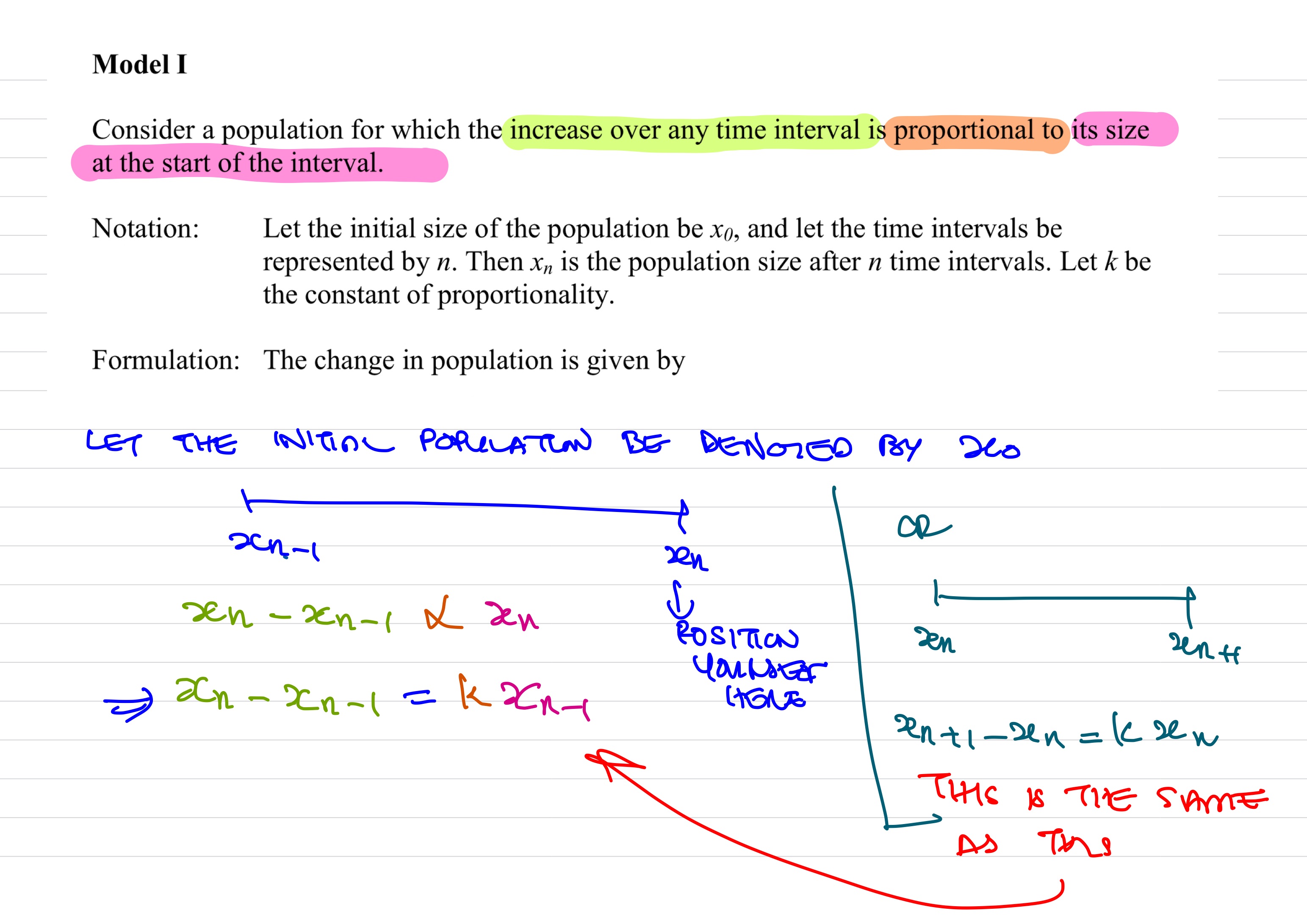
5. Model Problematization What if the system was set up as \[\begin{equation*} x_{n+1} - x_{n} = k x_{n} \end{equation*}\] instead?
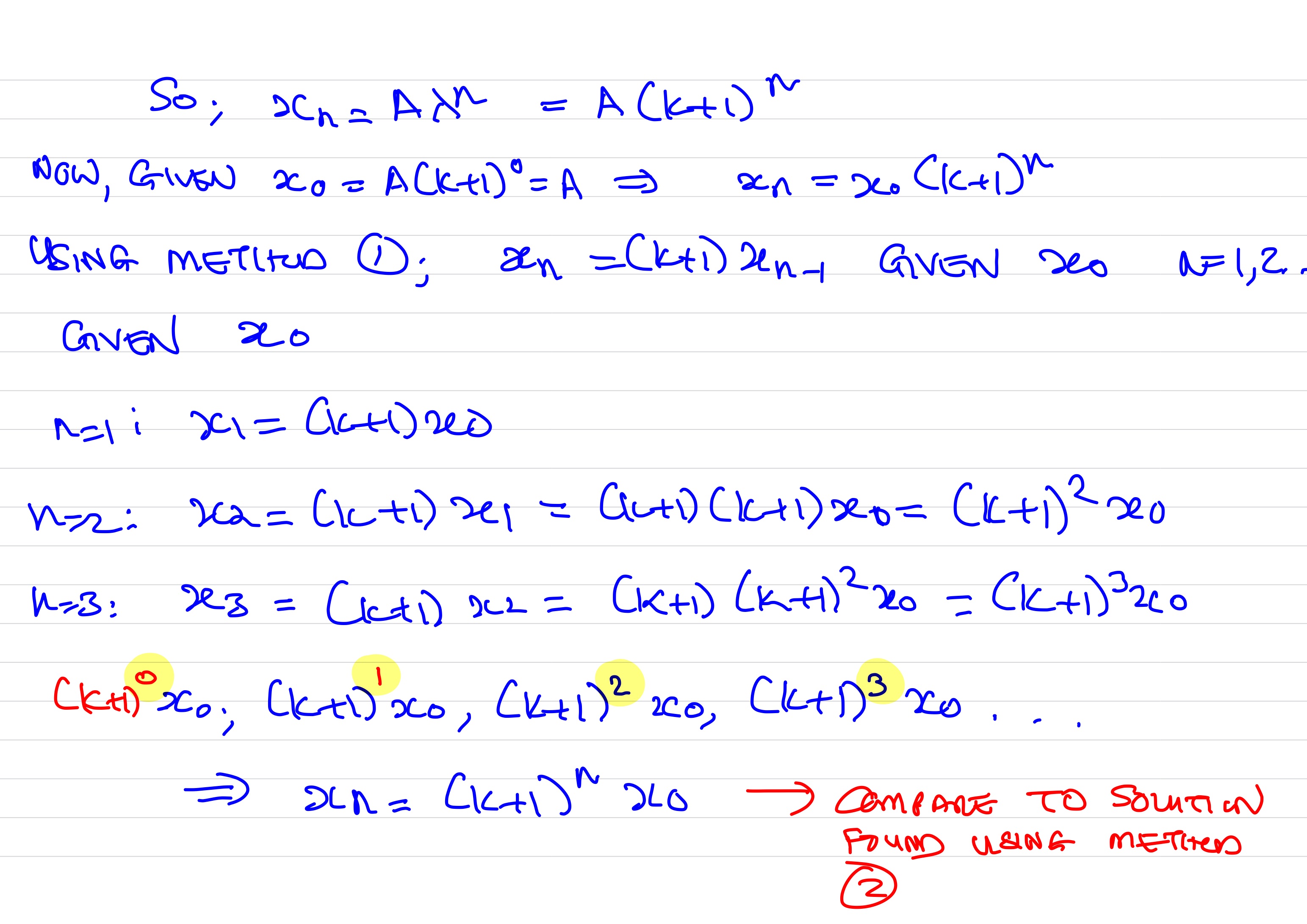
6. Model Solution It is convenient to rewrite the governing equation for this system as \[\begin{equation*} x_{n} = (k+1) x_{n-1}, \end{equation*}\] given \(x_0\), and \(n=1,2,\dots\)
We can solve this model using the direct brute force method of induction on \(n\) to yield, \[\begin{align*} x_{1} &= (k+1) x_{0}, \\ x_{2} &= (k+1) x_{1}=(k+1)(k+1) x_{0}=\left(k+1\right)^{2} x_{0},\\ x_{3} &= (k+1) x_{2}=(k+1)\left(k+1\right)^{2} x_{0}=\left(k+1\right)^{3} x_{0},\\ &\vdots\\ x_{n} &= \left(k+1\right)^{n} x_{0}. \end{align*}\] So, after \(n\) successive intervals, starting at \(n = 1\), the population is \[\begin{equation*} x_n = x_{0} \left(k+1\right)^{n}. \end{equation*}\]
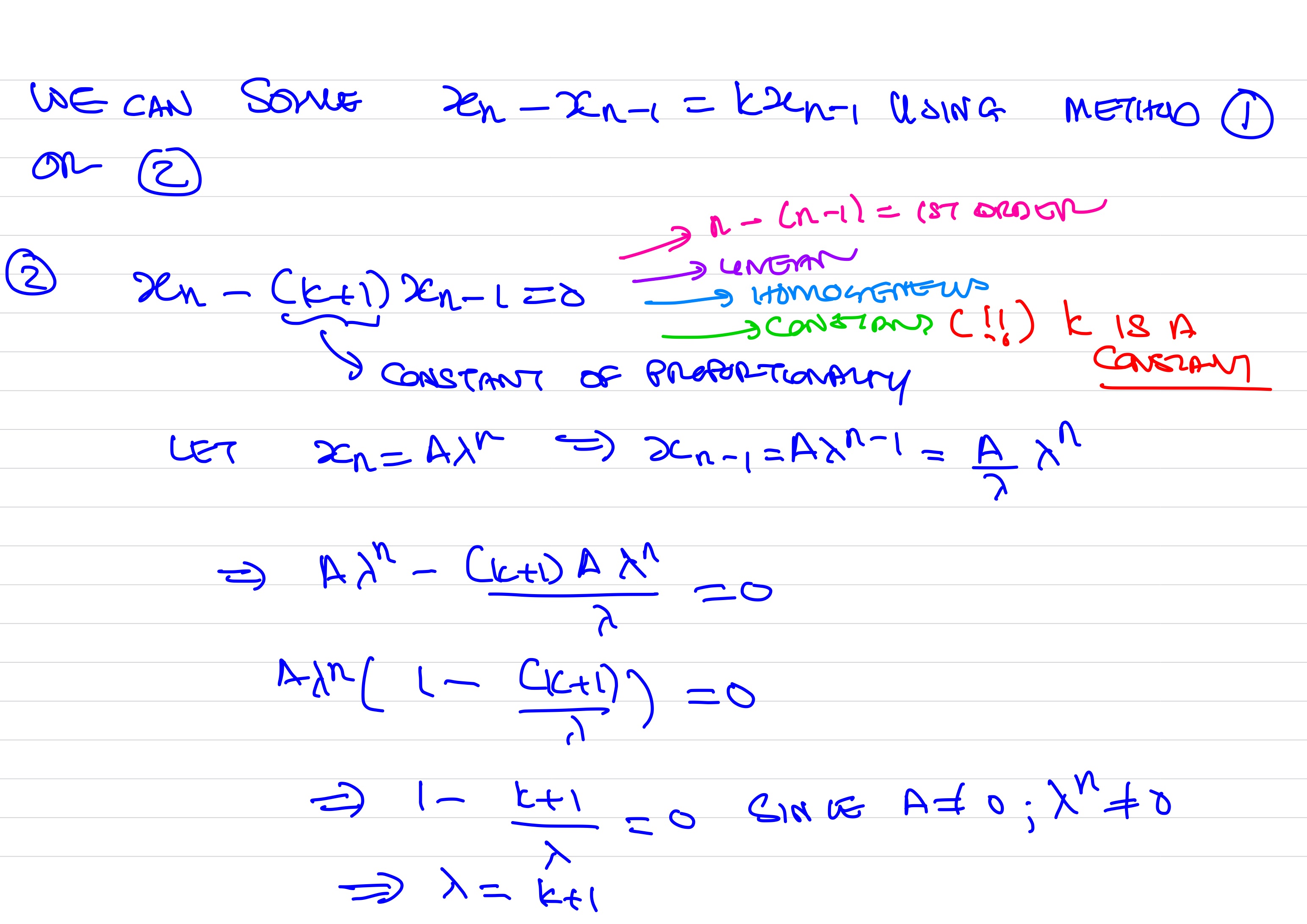
We can also solve the model by finding a general solution using the method of undetermined coefficients.
As done previous chapter, we begin with an initial trial solution of the form \(x_n = A\lambda^n\), and so \(x_{n-1}=A\lambda^{n-1}=\dfrac{A}{\lambda}\lambda^n\). Substituting \(x_n\) and \(x_{n-1}\) into the governing model gives that \[\begin{align*} A\lambda^n - (k+1) \dfrac{A}{\lambda}\lambda^n &= 0, \\ A\lambda^n\left(1-\dfrac{(k+1)}{\lambda}\right) &= 0. \end{align*}\] This implies that \[\begin{equation*} 1-\dfrac{(k+1)}{\lambda}=0 \end{equation*}\] since \(A \neq 0\) and \(\lambda^n \neq 0\). And so \(\lambda=k+1\). And so we have that \[\begin{equation*} x_n=A\left(k+1\right)^{n}. \end{equation*}\] Now given that when \(n = 0\), \(x_0 = \left(k+1\right)^{0}=A\). And so we have the general solution to be \[\begin{equation*} x_n=x_0\left(k+1\right)^{n}. \end{equation*}\]
7. Model Interpretation The change in population size is proportional to the size of the original population.
- If \(-1 < k < 0\), then the population size decreases for each iteration.
- If \(k = 0\), then the population size is constant.
- If \(k>0\), then the population grows with each iteration.
- If \(k < -1\), this does not give a realistic solution to this model - the model would have an oscillating population.
- Sketch the graph of \(x_n\) for \(k = -1, \: 0, \:1; \: -1 < k < 0; \: 0 < k < 1; \: k > 0\).
Next we consider a slight variation of Model 1.
Model 2: Discrete Population Growth Proportional to Change in Population Size
Consider a population where the change in population number over any time interval is proportional to the change in population number over the previous interval. What is the population size after \(n\) time intervals?
1. Problem Identification We want to find the population function \(x(n)\) for the population after \(n\) time intervals.
2. Assumption Specification Suppose the initial population has size \(x_{0}\).
3. Variable Classification Let \(x_{i} \equiv x(t_{i})\) denote the size of the population at time \(t_{i}\), the \(i\)-th time interval.
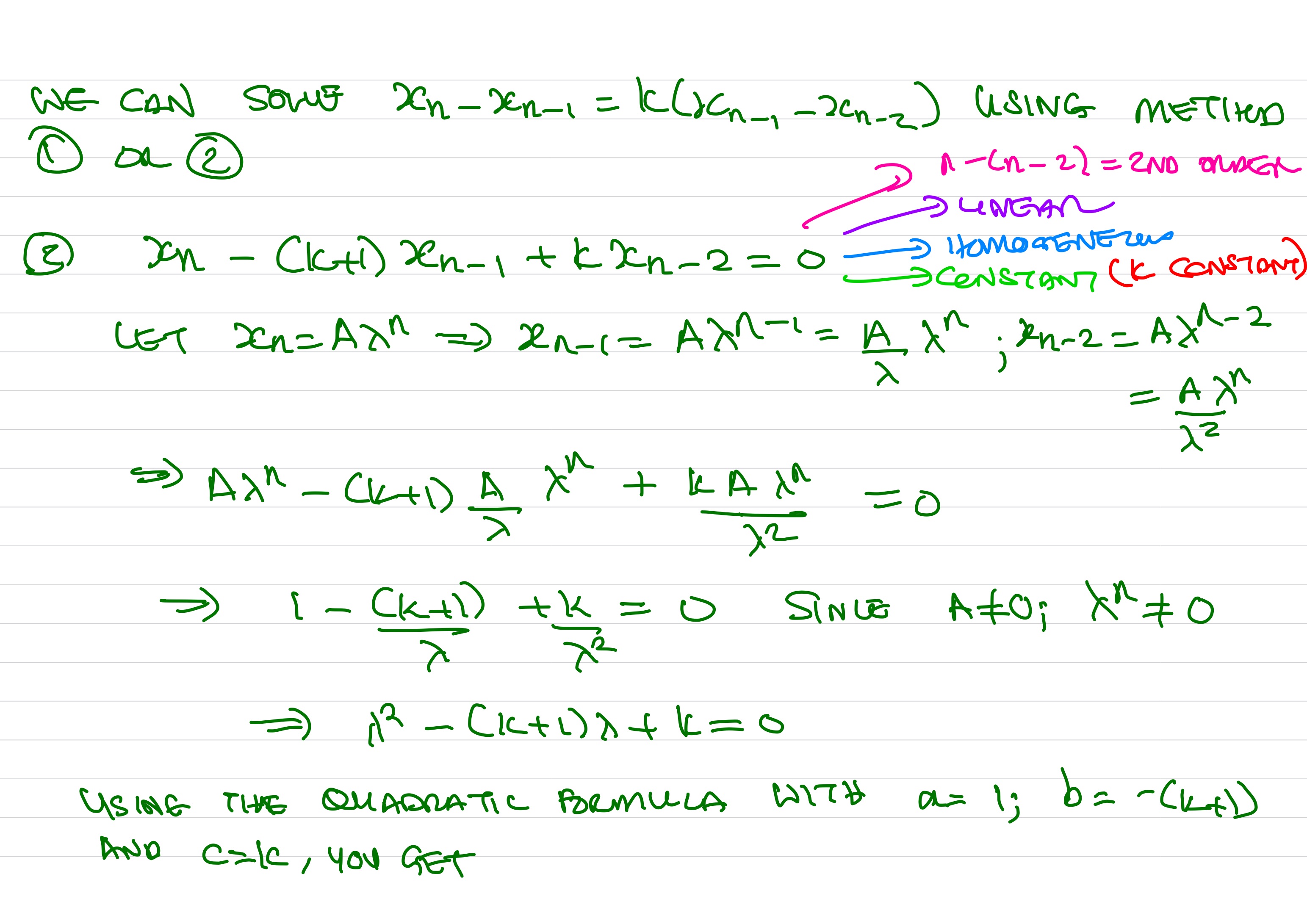
4. Model Construction Given this collection of assumptions, the change in population size across successive time intervals is then \[\begin{equation*} \left(x_{n} - x_{n-1}\right) \propto \left(x_{n-1} - x_{n-2} \right). \end{equation*}\] We can write this proportionality relationship as an equation \[\begin{equation*} x_{n} - x_{n-1} = k \left(x_{n-1} - x_{n-2} \right), \end{equation*}\] where \(k\) is the constant of proportionality. This equation relates sequence values at three different index values, \(n\), \(n-1\), and \(n-2\).
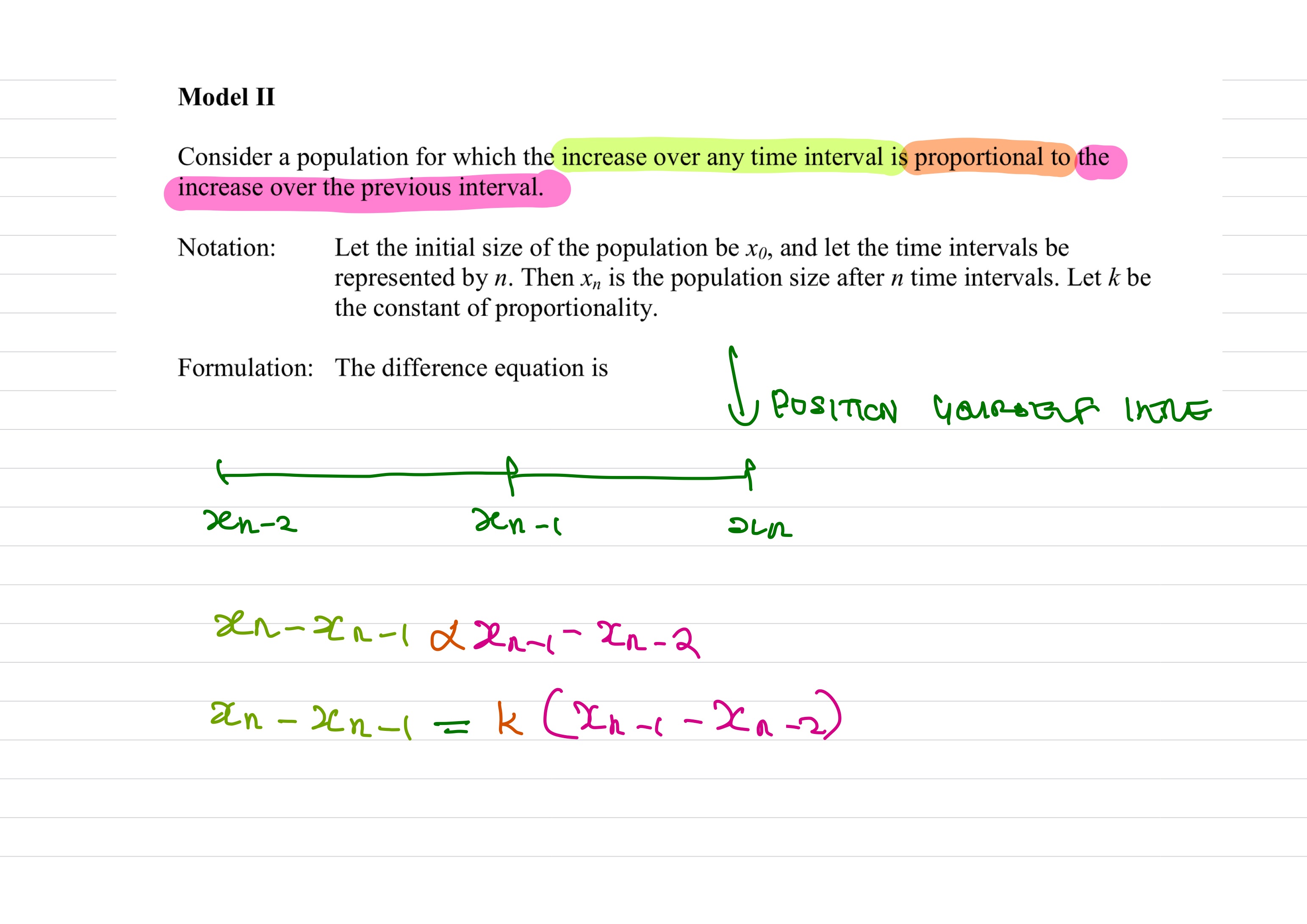
5. Model Problematization What if the system was set up as \[\begin{equation*} x_{n+1} - x_{n} = k \left(x_{n} - x_{n-1} \right), \end{equation*}\] or \[\begin{equation*} x_{n+2} - x_{n+1} = k \left(x_{n+1} - x_{n} \right) \end{equation*}\] instead?
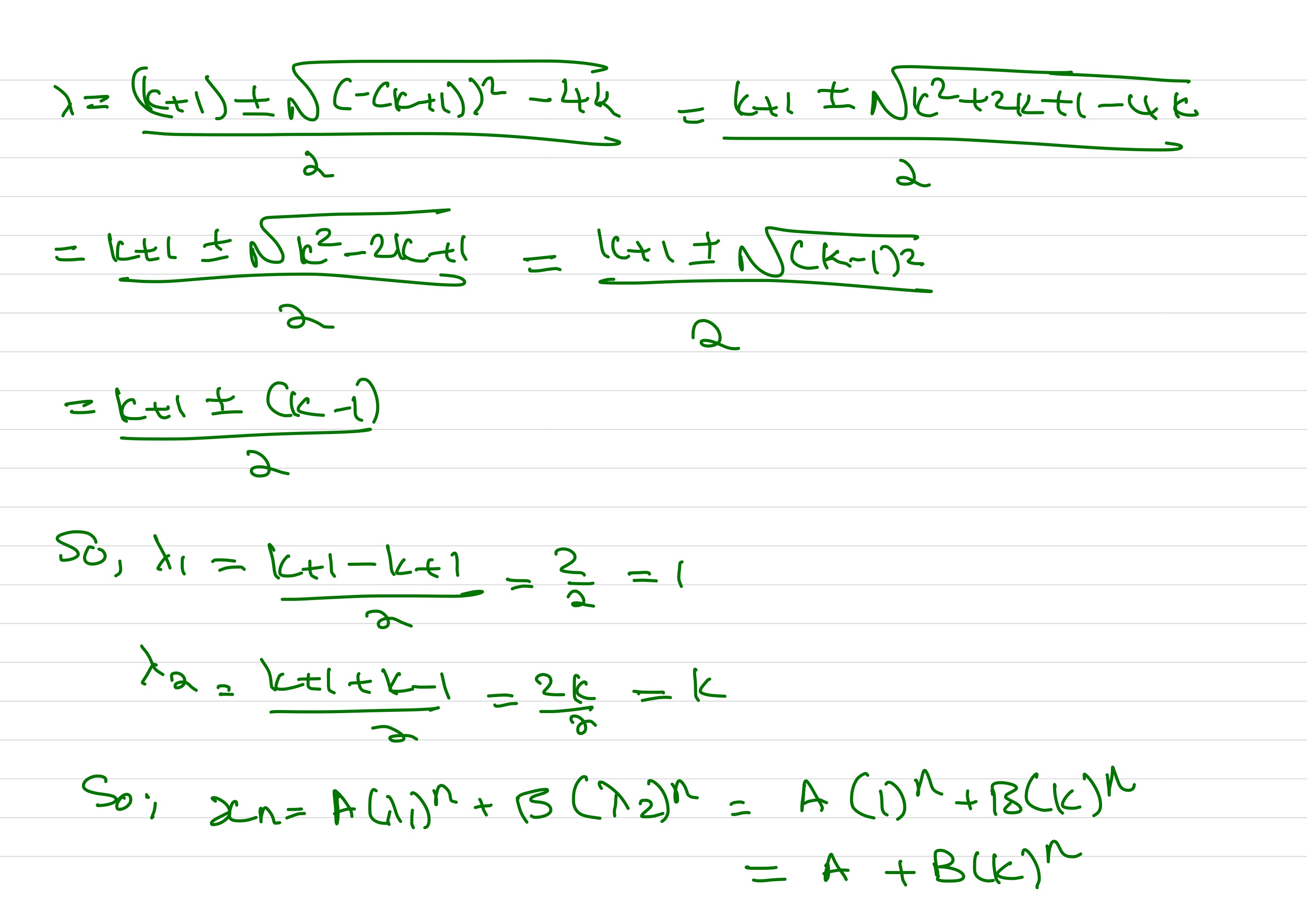
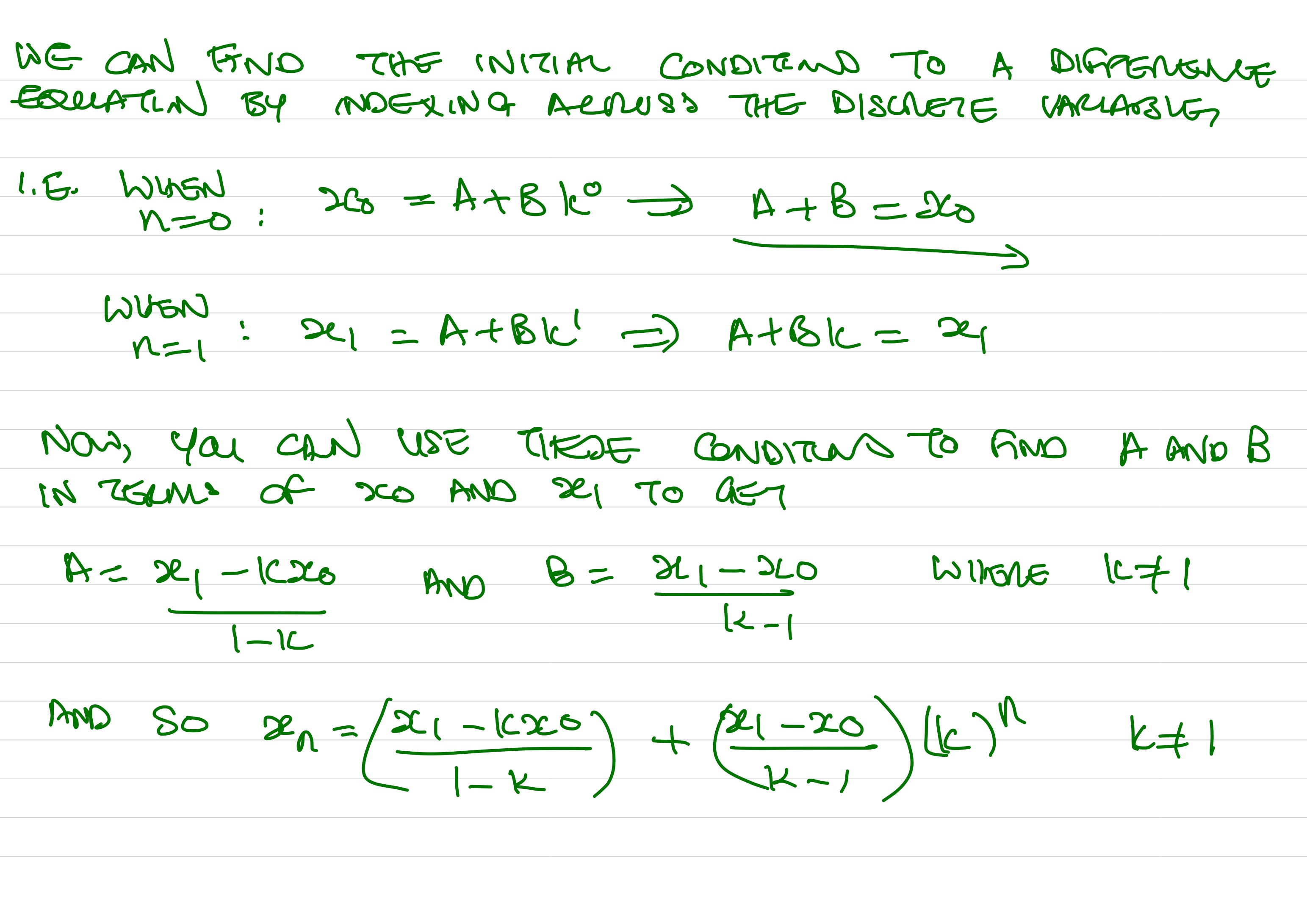
6. Model Solution We can solve the model by finding a general solution using the direct method or the method of undetermined coefficients.
 As is demonstrated in the above two models, small changes in one recurrence relation can bring about remarkable changes in the behaviour of a system.
Exercise:
Determine the nth term of the Fibonacci numbers \(1, 1, 2, 3, 5, 8, 13, 21, 34, 55, ....\)
Let \(P_n\) and \(D_n\) represent respectively the production and demand of a particular commodity at the end of any given year \(n\). Suppose that the change in production at the end of any year is proportional to the difference in production and demand at the beginning of that year (constant of proportionality \(\alpha > 0\)), and that the change in demand at the end of any year is proportional to the difference between production and demand at the beginning of that year (constant of proportionality \(\beta > 0\)). Assume that the production at the end of any year will go up/down if demand at the beginning of that year is greater/less than production at the beginning of that year, and that demand at the end of any year will go up/down if production at the beginning of that year is greater/less than, demand at the beginning of that year.
- Suggest a suitable mathematical formulation of this economic model.
- Derive the discrete functions \(P_n\) and \(D_n\) in terms of \(n\) assuming that \(\alpha = \beta = k\).
- Sketch, by inspection, the graphs of \(P_n\) and \(D_n\) for the following six cases: \(k = 0; \quad 0 < k < \frac{1}{2} ; \quad k = \frac{1}{2}; \quad \frac{1}{2} < k < 1; \quad k =1; \quad k > 1.\)
The “inbreeding coefficient” is the probability that two genes are identical by descent. If \(f_n\) is the inbreeding coefficient after \(n\) generations, it can be shown that \(f_{n+2} = \frac{1}{4} (f_n +2f_{n+1} +1)\). Find \(f_n\) given \(f_0 = f_1 = 0\).
It has been suggested that for self-fertilizing organisms, \(f_{n+1} = \frac{1}{2}(1 + f_n)\). Solve this for \(f_0 = 0\) and compare the result with that of the previous problem.
Selected Answers:
\(T_n=\dfrac{1}{\sqrt{5}}\left[\left(\dfrac{1+\sqrt{5}}{2}\right)^n-\left(\dfrac{1-\sqrt{5}}{2}\right)^n \right]\)
- \(P_n = P_{n-1} + \alpha(D_{n-1} - P_{n-1})\); \(D_n = D_{n-1} + \beta (P_{n-1} - D_{n-1})\)
- \(P_n = \frac{1}{2} (P_0 + D_0) + \frac{1}{2} (P_0 - D_0)(1 - 2k)^n\); \(D_n = \frac{1}{2} (D_0 + P_0)+ \frac{1}{2} (D_0-P_0)(1-2k)^n\)
\(f_n=1+\left(\dfrac{3\sqrt{5}-5}{10}\right)\left(\dfrac{1-\sqrt{5}}{4}\right)^n-\left(\dfrac{3\sqrt{5}+5}{10}\right)\left(\dfrac{1+\sqrt{5}}{4}\right)^n\)
\(f_n = 1 - \left( \frac{1}{2} \right)^n\)