Chapter 5 Computational Geometry
Content in this chapter was originally prepared and edited by Prof Ian Sanders and Prof Hima Vadapalli.
5.1 Summary Lecture
The video below summarises the content in this chapter. You may either watch it first, or read through the notes and watch it as a recap.
5.2 Introduction
While there are numerous classical computational geometry problems, we will consider just one in these notes. In particular, we will consider the closest pair problem: given the locations of \(n\) objects, find out how close the closest pair of these objects are together. The objects may correspond, for example, to parts in a computer chip, to cities on a map, to stars in a galaxy, or to irrigation systems. This is an example of a proximity problem. Other proximity problems include finding, for each point in the set, the closest point to it or the \(k\) closest points to it, and finding the closest point to a new given point.
Specifically, the problem definition is as follows.
Closest Pair Problem: Given a set of \(n\) points in the plane, find the distance between a pair of closest points. Each point \(p_i\) is represented as a pair of coordinates \((x_i, y_i)\).
5.3 Brute Force Approach
A straightforward solution is to check the distances between all pairs and to take the minimal one –– see for example the algorithm in below. To do the analysis of this algorithm, we choose a suitable “basic operation,” determine how often this basic operation is executed and then consider the algorithm’s asymptotic performance. A suitable basic operation for this algorithm is the number of comparisons between \(d\) and a newly calculated distance (or we could use the distance computations themselves). The algorithm does \((n−1)+(n−2)+(n−3)+ \ldots +2+1 = n(n−1)/2\) comparisons and similarly \(n(n − 1)/2 + 1\) distance computations.
A straightforward solution using recursion would proceed by removing a point, solving the problem for \(n − 1\) points, and then considering the extra point. An algorithm for this approach is given below. However, if the only information obtained from the solution of the \(n − 1\) case is the minimum distance between those, then the distances from the additional point to all other \(n − 1\) points must be checked. As a result, the total number of distance computations \(T(n)\) satisfies the recurrence relation \(T(n) = T(n − 1) + n − 1, (T(2) = 1)\), and we have already seen that \(T(n) = O(n^2)\).
5.3.1 Correctness
Having developed a solution to solve the problem we still have to convince ourselves that the solution method is correct. For these two algorithms a simple inductive proof will suffice. We will consider the iterative algorithm in this instance and prove that it returns the correct solution for any set of \(n\) points in the plane.
Proof:
Base Case: The base case of our proof is when there are only two points in the set. In this case, the distance between them is calculated directly. This is done in line 01 and again in line 04. The outer loops runs from 1 to 1 and so is executed only once, the inner loop runs from 2 to 2 and so is also only executed once. This means that we calculate the distance between points 1 and 2 and this is the only answer that \(d\) can take on. Our base case is correct.
Induction Hypothesis: Our induction hypothesis is that the algorithm works correctly for any set of \(k − 1 > 2\) points in the plane.
Inductive Step: We must now show that the algorithm works for any set of \(k\) points. By our induction hypothesis the algorithm works if we have \(k − 1\) points. The extra work done in the algorithm is that each time the inner loop executes there is one extra distance computation –– to check the distance between the point being considered (as referenced by the index of the outer loop) and the \(k\)th point. If this computation results in a smaller distance than the result of all the other steps in the inner loop (which our induction hypothesis tells us is the correct solution), then \(d\) will be updated to reflect this; otherwise, \(d\) will not be updated. The outer loop also executes one extra time resulting in one extra execution of the inner loop, to calculate the distance between the \(k − 1\)th and \(k\)th points and to compare this distance to the shortest distance computed so far and to update \(d\) if necessary. The induction hypothesis tells us that all of the distances between the 1st to \(k − 1\)th points are computed and compared (and \(d\) updated if necessary) and we have shown that the distance from each point to the \(k\)th point is computed and compared (and \(d\) updated if necessary) and thus can be confident our solution method is correct.
The proof for the recursive algorithm is similar.
A final step in our consideration of this algorithm would be to determine whether this algorithm is optimal. It isn’t! There is a better algorithm which we consider next.
5.4 Divide and Conquer Approach
We looked at a straight forward solution to the problem of finding a pair of closest points in the previous section. That algorithm is \(O(n^2)\). Can we do better?
In this section of the text we consider a divide-and-conquer approach to solving the problem. Instead of considering one point at a time as we did in our recursive algorithm above, we will divide the set into two roughly equal parts. When we do this splitting of the input data into two parts we want to do it in a manner which will save us work later on. In this case we would not just want to divide the input data into two sets of points each of size roughly \(n/2\), but we would like to make use of the geometry of the problem by dividing the input set into points which are in some sense close together.
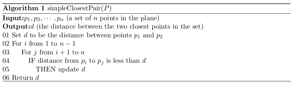
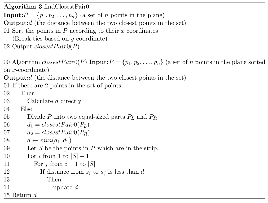
One approach to doing this is to divide the plane into two disjoint parts each containing about half of the original set of points. We can do this by sorting all of the points according to their \(x\) coordinates and then dividing the plane by a vertical line that splits the set into two roughly equal sets (see figure below). Note that this initial sorting needs to be performed once only — it is considered as preprocessing.
Figure 5.1: The closest pair problem — dividing the data
Note that it makes the problem slightly easier to understand if we assume that \(n\), the number of points, is a power of two because this means that the set can always be split into two equal parts. It is, however, relatively simple to generalise the algorithm to work for arbitrary \(n\). Note too that we will only find the minimal distance between the points — figuring out the actual two closest points will be straightforward from the algorithm.
The approach which the algorithm takes is essentially that if \(P\) is a set of \(n\) points, then we first divide \(P\) into two equal-sized subsets, \(P_L\) and \(P_R\) , as described above. We then find the closest distance in each subset by recursion. Then we build up the complete solution by “merging” the answers from the two subsets. To do this merging, we have to determine if there are two points, one on either side of the dividing line, which are closer together than the closest points in the two subsets.
Clearly, this dividing into two subsets, recursively solving the problem for each subset and then building the combined solution happens at each level of recursion. Dividing each subset into two smaller subsets at each level of recursion can be done in constant time if the points are maintained in sorted order after the original sorting based on \(x\) coordinate. The limiting case for this algorithm is when the subsets contain only 2 points and the distance between them can be calculated directly.
Finding the distance between the closest points when the merging is being done requires a bit more thought.
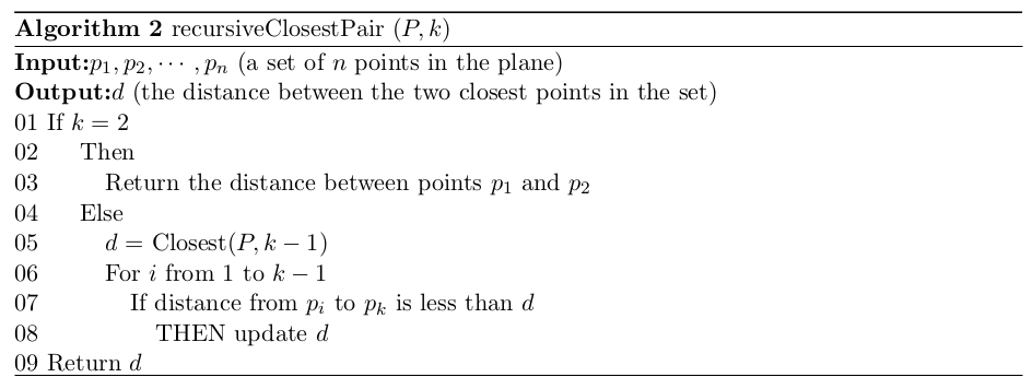
Suppose that at some level of recursion, the minimal distances in the left and right parts have been found. Let the minimal distance in \(P_l\) be \(d_1\) , and in \(P_r\) be \(d_2\) , and assume without loss of generality, that \(d_1 \le d_2\). Then the smallest distance (that we know about so far) is \(d = d_1\). We need, however, to find the closest distance between all the points at the current level of recursion; that is we have to see whether there is a point in \(P_l\) which is a distance \(< d\) from a point in \(P_r\) . To do this, we make use of the insight that if two such points existed then each point would have to be no further than \(d\) from the dividing line between the two subsets. This means that we would only need to consider points which fall in the “strip” of width \(2d\) centred on the dividing line (see figure below). No other point can be of distance less than \(d\) from points in the other subset. See Algorithm 3 for a first attempt at describing this algorithm.
Figure 5.2: The closest pair problem – the ‘strip’ around the dividing line
Using this approach we can, if we are lucky, eliminate many points from consideration in the merging phase – for example in Figure 5.2 half of the points would have been eliminated. In the worst case, however, all of the points could still fall inside the strip (see Figure 5.3) and we would then essentially be repeating our brute force algorithm at each level of the recursion. This would give us a recurrence relation of \(T(n) = 2T(n/2)+O(n^2)\) (solve this as an exercise) which isn’t an improvement on the straightforward algorithm.
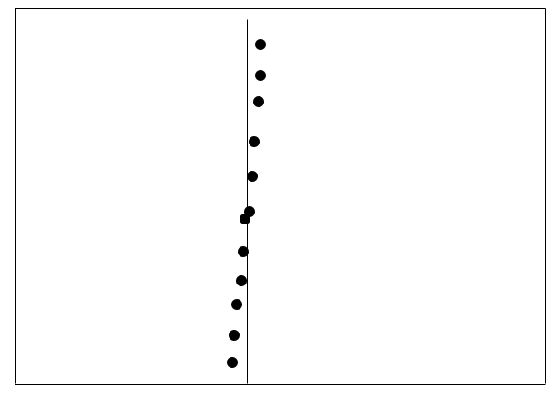
Figure 5.3: All points would fall into the strip over the dividing line
It turns out that we can do better than this though – we never actually have to look at all of the points which fall inside of the strip. This is because for any point \(p\) in the strip, there can only be a few points on the other side whose distance to \(p\) can be smaller than \(d\). To see this note that all the points in each strip are at least \(d\) apart — \(d\) is the smaller of \(d_1\) and \(d_2\) which were the smallest distances to the left and right of the dividing line respectively. If any points in the strip but not across the dividing line were closer together than \(d\) then \(d_1\) or \(d_2\) would have been smaller and so \(d\) would have been smaller.
Suppose without loss of generality that \(p_l\) (a point to the left of the dividing line) and \(p_r\) (a point to the right of the dividing line) are actually the two closest points. We know that the distance between \(p_l\) and any other point to the left of the dividing line must be at least \(d_1\) and we know that the distance between \(p_r\) and any other point to the right of the dividing line must be at least \(d_2\) . This means that there are areas in the two half planes where other points from the same half plane could not appear — in this case in the interior of the circles of radius \(d\) centred at \(p_l\) and \(p_r\) as shown in the Figure 5.4. Note how \(q_r\) is not within the circle of radius \(d\) of \(p_r\).
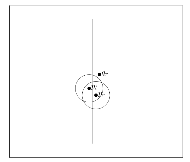
Figure 5.4: The closest pair problem — if \(p_l\) and \(p_r\) are the closest pair of points then other points on the left cannot appear within a circle of radius \(d\) of \(p_l\) and other points on the right cannot appear within a circle of radius \(d\) of \(p_r\)
What we would like to do is to use this information to find a way to cut down the number of points that each point in the strip around the dividing line is actually compared to. Clearly if the closest points are actually in the strip then two points — one on either side of the line — must be less than \(d\) apart. So for each point which is close to the dividing line we would need to consider if any points on the other side of the dividing line fall within \(d\) of that point. In Figure 5.4, \(p_r\) falls inside the circle of radius \(d\) of \(p_l\) but \(q_r\) does not. What we would like to do is to place a limit on how many such points there could possibly be. Then, for each point, we would only have to consider that number of points instead of all of the other points in the strip.
To simplify the problem a bit, let us just consider points which have \(y\) coordinates \(\le d\) apart — any points which have \(y\) coordinates more than \(d\) apart definitely should not be considered any further. Note that on either side of the dividing line and within the strip on that side of the line, we can have groups of at most four points which have \(y\) coordinates \(d\) apart. These groups of four points must be positioned at the corners of squares of dimensions \(d \times d\) where one edge is on the dividing line and the opposite edge is \(d\) from the dividing line and parallel to it. If two such groups of points (one on either side of the dividing line) were arranged so that the points on the dividing line were coincident, then we would have a rectangle of size \(2d \times d\) where all of the points are \(d\) apart in \(y\) coordinate. This is the maximum number of points which could meet this condition.
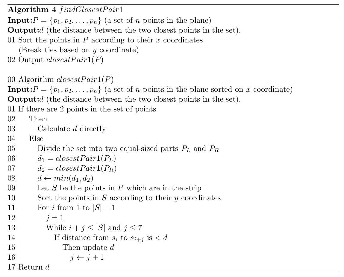
So if we consider the points in the strip in order of increasing \(y\) coordinates (breaking ties on increasing \(x\) coordinate) then each point, as we encounter it, could have at most 7 points, which come after it in the sorted order, that are a \(y\) distance of \(\le d\) from it. So to determine the closest pair inside the strip, we first discard all of the points outside of the strip around the dividing line. We then sort the remaining points on \(y\) coordinate. Thereafter we need to check each point against only a constant number of its neighbours in the \(y\) sorted order (instead of against all \(n − 1\) points). The improved algorithm is given in Algorithm 4.
Let us now consider the running time of this improved algorithm. The preprocessing — sorting based on \(x\) coordinate – takes \(O(n\lg n)\) time but is done only once. In the main processing phase, the set of points is split into two which takes constant time. Then two subproblems of size \(n/2\) are solved. Then, to calculate the final answer, the points outside of the strip are eliminated in \(O(n)\) time. Sorting according to the \(y\) coordinates then takes \(O(n \lg n)\) time. Then it takes \(O(n)\) time to work through the sorted list of the points inside the strip and to compare each point to a constant number of its neighbours in the sorted list. This gives the recurrence relation: \(T(n) = 2T(n/2)+O(n \lg n), T(2) = 1\). It turns out that the solution of this recurrence relation is \(T(n) =O(n \lg^2 n)\). This is asymptotically better than a quadratic algorithm, but we still want to do better than that.
5.5 An \(O(n \lg n)\) Algorithm
The algorithm in Algorithm 4 sorts the points in the strip based on their \(y\) coordinates (in \(O(n \lg n)\) time) during the combining step at every level of recursion. This is more expensive than the linear passes we have to make to eliminate points outside of the strip and to scan the points inside the strip to see if there are points closer together than the closest points in each subset. We have to do the scan but can we do the sorting more efficiently to make our overall algorithm more efficient?
We know from the mergesort algorithm that we can merge two sorted lists in linear time (by making a single pass through the lists). So we could use the mergesort approach to do the sorting more efficiently. At the limiting case of the algorithm we would find the distance between the two points and sort them based on their \(y\) coordinates and then return \(d\) and the sorted sublist. So at each level of recursion — where we are combining the solutions — we only have to merge and not sort. Since the merging can be done in \(O(n)\) time, the recurrence relation becomes \(T(n) = 2T(n/2)+O(n), T (2) = 1\), which implies that \(T(n) = O(n \lg n)\). The revised algorithm is given in Algorithm 5.
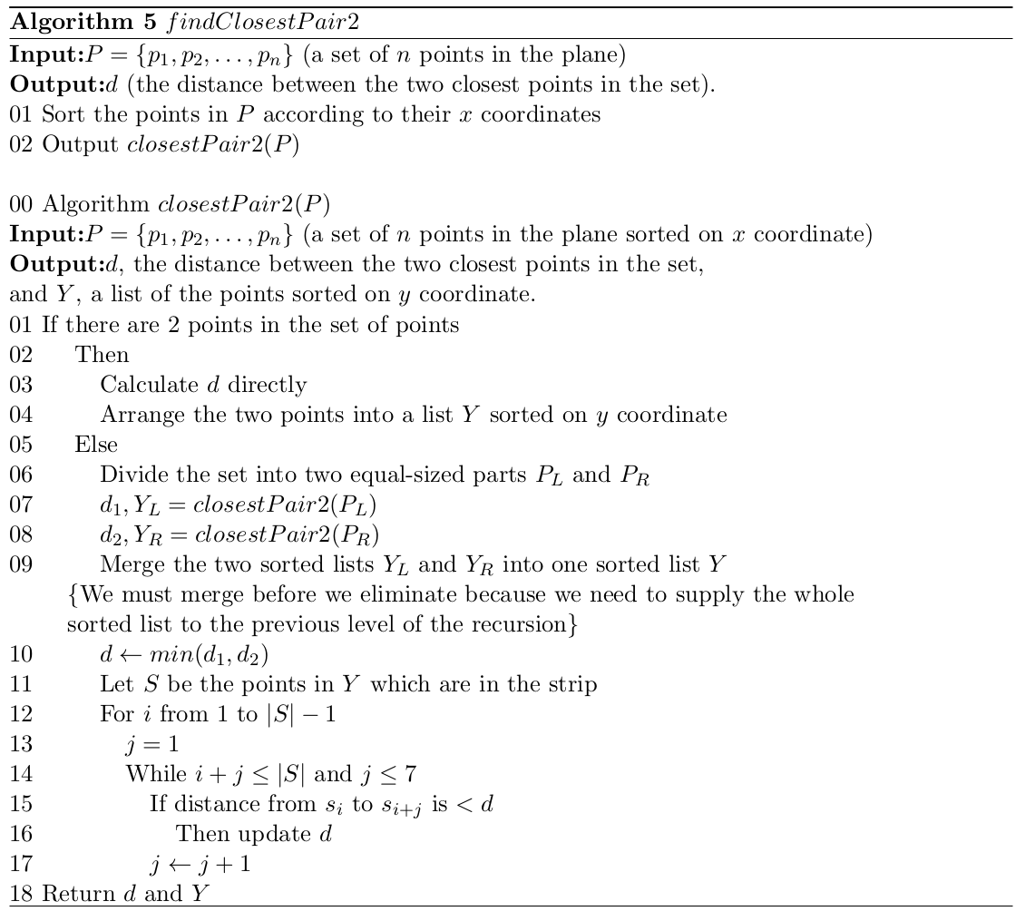
Note that throughout the preceding two sections we assumed that \(n\) was a power of \(2\). The algorithm will work for general n provided that the limiting case is changed to there being \(\le 3\) points in the set of points at any level of the recursion. Calculating the minimum distance between three or fewer points and sorting the list of three or fewer points can still be done in constant time and so the efficiency of the algorithm is not affected.
5.5.1 Optimality
The interested (and dedicated) reader is referred to Preparata and Shamos, Computational Geometry, Springer 1993.
5.5.2 Correctness
The correctness of the solution method can be proved by induction on the powers of \(2\) in the case where \(n = 2^m\). Here the algorithm clearly works if \(m = 1\) — the distance between the two points is calculated directly.
If the result holds for \(m = k − 1 > 1\), then we need to show that the result from \(m = k\) can be correctly determined from the two solutions of size \(2^{k−1}\). Eliminating the points outside the “strip” will not cause a problem as they have already been considered to find the smallest distance in each sub-problem, and they are too far away from points on the other side of the dividing line to be considered here. Points on one side of the dividing line in the strip could possibly be paired with points on the other side of the dividing line to give a closest pair. If we consider all such pairs, then clearly we will not miss the pair which is closer together than the already determined closest pair, but we do not consider all such pairs.
We have, however, argued that at most eight points can be arranged in a group where the difference in \(y\) coordinate values between each pair of points is at least \(d\). Thus each point in such a group needs only to be checked with its seven neighbours. If the points are arranged in \(y\) coordinate order and we scan from smallest \(y\) value then each point only needs to be checked against the next seven points in the list. Points outside of this range would have to have a \(y\) coordinate distance greater than \(d\) and thus could not be a distance less than \(d\) from the current point. The algorithm will thus find any pair of points which are less than \(d\) apart and will pick the smallest of these new distances as the result for a set of points of size \(m = 2^k\) . The algorithm is thus correct for all sets of points where the number of points is a power of two.
If \(n\) is not a power of \(2\) then the only other thing we have to worry about is the limiting case of the recursion. We do not want to have a set of points of size \(1\), as the minimum distance between the points would be undefined in such a case. Setting the limiting case as \(\le 3\) takes care of this case — any limiting size set will have either 2 or 3 points in it — at some small extra cost which does not affect the order of complexity of the algorithm.
5.6 Additional Reading
- Introduction to Algorithms (Chapter 33), Cormen, Leisersin, Rivest and Stein, 3rd ed.
- https://www.youtube.com/watch?v=0W_m46Q4qMc/