Chapter 1 Searching
Content in this chapter was originally prepared and edited by Prof Ian Sanders and Prof Hima Vadapalli.
1.1 Summary Lecture
The video below summarises the content in this chapter. You may either watch it first, or read through the notes and watch it as a recap.
Computers are tools which are used to solve problems for us. One of the things that computers are very useful for is for storing vast amounts of data of various forms. In order to make the best use of the machines and be able to access the data easily we need efficient ways to search for particular items of data. To illustrate this let us look at a list of numbers.
| Position | 0 | 1 | 2 | 3 | 4 | 5 | 6 | 7 | 8 | 9 | 10 |
|---|---|---|---|---|---|---|---|---|---|---|---|
| 3 | 17 | 24 | 12 | 18 | 89 | 45 | 87 | 15 | 49 | 30 |
Typically we could be asked to find
- The position of largest element
- The element with value = 9
- The number of elements with value = 15
The question then arises: How do we do this? In the next section of the text we will consider an algorithm for determining where a given number, the key, occurs in a list of numbers. This is analogous to point 2 above.
1.2 Linear Search 1
Our problem here is to determine where a particular number, the key, appears in a given list of numbers. We will first assume that the key is in the list of numbers but the algorithm can be modified to take into account the case where the key is not in the list (we will consider that case a bit later).
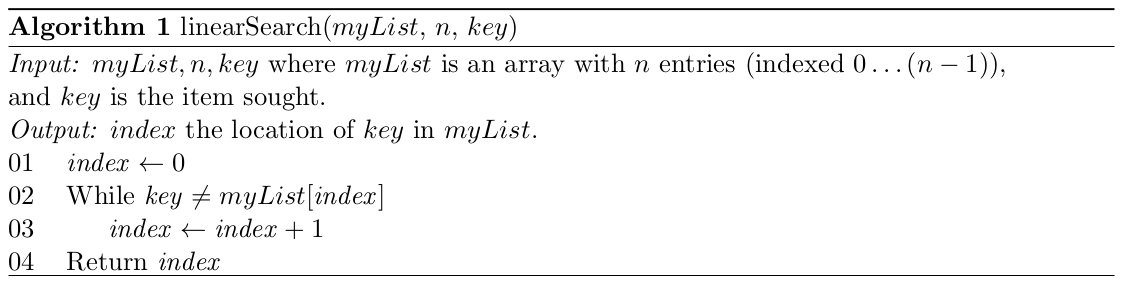
In our search we start at the first element in the array and check it against the key. If it matches the key then we have found the number that we are looking for and we can terminate our search. If it is not the number that we are looking for, we move on to the next element in the array and repeat the process. We carry on doing this until we find an element which has the same value as the key. The algorithm for the linear search is given in Algorithm 1. (Note that this algorithm would be called by another algorithm which has read in the list of numbers and stored them in an array and has also determined which number will be looked for in the list.) This search is also called the sequential search.
1.2.1 Correctness
Now we have an algorithm which we believe will return the correct answer for any valid input. We should still, however, prove that the algorithm is correct. We can do this by means of a simple direct proof.
Theorem 1. linearSearch works correctly for any valid input.
Proof
The first line of the algorithm sets index to have the value 0 — that is, it sets \(index\) to point to the first element in the list of numbers (position 0 in the array). The \(while\) loop condition is then tested. There are two cases to consider. If \(key = myList[0]\) (the number we are looking for is the first number in the list) or if \(key \neq myList[0]\) (the number we are looking for is not the first number in the list). If the first case holds the algorithm will not go into the body of the loop and 0 will be returned. This would be the correct answer. If the second case holds then \(index\) would be incremented by 1 (to consider the second number in the list – position 1 in the array). The \(while\) loop condition would then be tested again. Once again the two cases would be considered and either the number would be found in which case the while loop would not be re-entered and the algorithm would return 1 which would be the correct answer. If the number is not found then \(index\) would be incremented again and the loop condition would be tested again. This would continue until a list position is found which contains a value equal to \(key\). This must happen as we know that such a value is in our list and because our list is stored in an array indexed from \(0\) to \(n − 1\) and we start searching at 0 and increment by exactly 1 each time we will consider every array position in turn. Our algorithm will thus return the correct answer.
1.2.2 Complexity
We will now look at the complexity of our searching algorithm. In this algorithm, the number of comparisons between the key and the value stored at some position in the list that the algorithm does is a good description of the amount of work the algorithm does and thus is an appropriate “basic operation” to use in our analysis. So to find the complexity function for the linear search, we will count the number of such comparisons the algorithm makes in order to find the key in the list of numbers. This algorithm clearly has a best and worst case. If the number we are looking for is the first number in the list (irrespective of the length of the list) then we will get a match straightaway. On the other hand if we have to work the whole way through the list and the number we are looking for is in the last position in the list then we will do much more work. So we do different amounts of work depending on where in the list the key appears.
1.2.2.1 Best case analysis
What is the best case for the linear search? In other words, when does the linear search make the lowest number of comparisons for a list of length \(n\)?
If the key is in the first position in the list (the first element in the array – in position 0) then we get an immediate match. This means we only test the condition in the while loop once. This is the best case for this algorithm. In this case our complexity function \(g_B(n) = 1 \cdot k\) where \(k\) is the cost of a comparison of the key with a list element.
1.2.2.2 Worst case analysis
What is the worst case for the linear search? In other words, when does the linear search make the highest number of comparisons for a list of length \(n\)?
If the key is in the last position in the list (that is, the key is the last element in the array) then we only get a match when we test the element in position (n − 1) of the array. That is, when \(index = (n − 1)\) and the condition \(key \neq myList[index]\) is false (\(key = myList[index]\)). This means we test the condition in the while loop once for each element in the array. If the array has \(n\) elements (numbered from 0 to \((n − 1)\)) then the condition is tested \(n\) times (there are \(n\) comparisons of the key with an array element). This is the worst case for this algorithm. Here g\(_W (n) = n \cdot k\).
1.2.2.3 Average case analysis
Let us now consider the average case for the linear search algorithm. Recall that when we are trying to consider the average case analysis for an algorithm, we look at the various forms of inputs which could occur and the probability of each of these inputs occurring. The average case complexity function for some algorithm is then given by \(g_A(n) = \Sigma_{I \in D_n} p(I) \cdot t(I)\) where \(D_n\) is the set of all possible forms of inputs of size \(n\) for the algorithm, \(p(I)\) is the probability of an input \(I\) occurring and \(t(I)\) is the cost of processing (or the time taken to process) that input instance.
For simplicity we assume in our analysis that the key appears exactly once in the given list of numbers and is equally likely to appear in any position in the list.
There are \(n\) possibilities for finding key – the element which matches the key could be in any of the \(n\) positions in the array. Thus there is a probability of \(1/n\) that the key could be in a particular position in the array. Let \(I_i\) represent the input instance where the key appears in the \(i\)th position in the array, then \(p(I_i) = 1/n\).
To find the match requires \(i + 1\) comparisons, \(0 \le i \le (n − 1)\), if the key is in position \(i\). That is \(t(I_i) = i + 1\). Therefore the expected number of comparisons is
\[ g_A(n) = \sum_{i=0}^{n-1} p(I_i) \cdot t(I_i) = (1/n) \cdot (1 + 2 + \ldots + n) = (1/n)\cdot n(n+1)/2 = (n+1)/2. \]
Therefore, \(g_A(n) \in O(n)\).
1.2.3 Optimality
We now need to consider the optimality of our linear search algorithm.
First we note that any problem has some minimum amount of work which must be done in order to solve it. An algorithm is optimal if, in the worst case, it performs as many basic operations as are required to solve the problem.
So in order to determine whether an algorithm (which we believe is efficient) is optimal, we first have to establish a lower bound on the number of operations needed to solve the problem. The problem that we are dealing with here is to determine the position of a number in a list of numbers by doing comparisons of \(key\), the number we are looking for, with numbers in various positions in the array. We need to find a lower bound for a problem in this class. That is, we need to find a bound on the number of such comparisons which must be done by any algorithm to solve this problem in this way. Here we are saying that for any algorithm which solves the problem in this way there must be at least one input instance which requires at least this much work.
We can find a lower bound for this problem by a simple adversary argument. If we assume that the numbers are distinct and we know that one of the numbers in the list is equal to key then \(n − 1\) numbers are not equal to \(key\). This means that an adversary could build up a “bad” input instance (in fact an input instance which is as bad as possible) for any algorithm which solves this problem. It would do so by simply assigning a value which is not equal to \(key\) for each position in the list which is being tested until there is only one position left where \(key\) could be. The adversary would then have to assign the value of \(key\) to that position in the list. This means that for any algorithm an adversary could force the algorithm to do at least \(n\) comparisons of \(key\) with values in the array. The lower bound for this problem is thus \(n\). The worst case for our algorithm is also \(n\) and so our algorithm can be taken as optimal among the group of algorithms that use sequential order for searching.
1.3 Linear Search 2
In the algorithm above we assumed that the number we were looking for was known to appear somewhere in the list of numbers. Suppose now that this is not the case – the number might not be in the list at all. For simplicity we will assume that there are no duplicates of key in the list – it either does not appear or it appears exactly once. How do we have to change the algorithm and how does the analysis change?
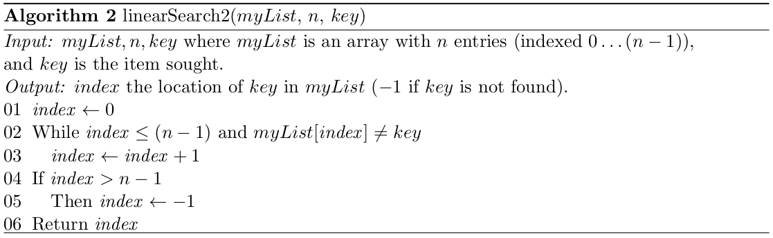
The main change to the algorithm is that, because the number might not be in the list, we have
to deal with the case where we get to the end of the list without finding the key. The condition
that is tested in the \(while\) loop of algorithm linearSearch2 takes this into account.
First there is a test to see if the current index into the array is within the range of where the
list is stored and only if this is true is the value in the current position of the list compared to
the key. The loop would terminate if either of these conditions was not true. After the loop
has terminated, the algorithm determines whether the loop terminated because all the numbers
had been considered and the end of the list has been reached, or whether the key has been found.
1.3.1 Correctness
Now we have an algorithm which we believe will return the correct answer for any valid input. We should still, however, prove that the algorithm is correct. We can do this by means of a simple inductive proof.
Theorem 2. linearSearch2 works correctly for any valid input.
Proof
Base case:
Let the length of the list be \(a = 1\), that is there is one element in the list. Then that element will be stored in position 0 in the array. The algorithm will first set \(index\) to be 0 and then will test the condition in the \(while\) loop. The first part of the condition (\(index \le (n − 1)\)) will be satisfied (\(0 \le 0\)) and so the second part of the condition will be tested. There are two cases to consider. If \(key = myList[index]\) (the number we are looking for is in the list) or if \(key \neq myList[index]\) (the number we are looking for is not in the list).
In the first case the algorithm will not go into the body of the \(while\) loop and the statement after the \(while\) loop will be executed next. The test in this statement will not be satisfied so the value of \(index\) will not be changed. It will remain as 0. The algorithm will then return the value of \(index\) which is 0. This is the position of the number (which is equal to the key) in the list and so the algorithm returns the correct answer.
If the second case holds then the algorithm would go into the body of the loop which would increment \(index\) to 1. The condition of the \(while\) loop would then be tested again. Here the first part of the condition would not be true (\(index = 1 > 0 = (1 − 1)\)). The loop would be terminated and the statement after the loop would be executed, the condition tested would be true and \(index\) would be set to −1. This value would then be returned by the algorithm. This is the correct answer. Thus our algorithm works for a list of length 1.
Induction hypothesis:
Assume now that the algorithm works for a list of length \(k − 1\) where \(k > 1\). This means that if we search for some number in the list then the algorithm will return the position of that number in the array if the number is in the array and will return −1 otherwise.
Inductive step:
We now need to show that the algorithm would work for a list of length \(k\). That is if we search for a number which appears in some position \(j\), \(0 \le j \le k − 1\) in the list of length \(k\) then the algorithm will return \(j\) and if the number is not in the list then the algorithm will return −1.
If the number appears in a position \(j, 0 \le j \le k − 2\) then by our induction hypothesis the algorithm will return the correct answer – this is effectively the algorithm working on a list of length \(k − 1\). If the number appears in position \(j = k − 1\) then the condition \(index \le (k − 1)\) and \(myList[index ] \neq key\) will be true for the first \(k − 1\) elements (positions 0 to \(k − 2\)). This follows from our induction hypothesis applied to the case when we consider a list of length \(k − 1\) which does not contain key. When \(index = (k − 2)\), the body of the loop will increment index to \(k − 1\) and the condition of the while loop would then be tested again. The first part of the condition (\(index \le (k − 1)\)) will be satisfied (\(k − 1 \le k − 1\)) and so the second part of the condition will be tested. There are two cases to consider. If \(key = myList[index]\) (the number we are looking for is in the list) and \(key \neq myList[index]\) (the number we are looking for is not in the list).
In the first case the algorithm will not go into the body of the while loop and will then return the value of index which is \(k − 1\) which is the position of the number in the list. If the second case holds then the algorithm would go into the body of the loop which would increment index to \(k\). The condition of the while loop would then be tested again. Here the first part of the condition would not be true (\(index = k > (k − 1)\)). The loop would be terminated and the statement after the loop would be executed and index would be set to −1 which would be returned by the algorithm. Thus our algorithm works for a list of length \(k\).
Thus by the principle of mathematical induction our result is proved.
1.3.2 Complexity
Let us now consider the efficiency of our modified algorithm. Once again our basic operation will be a comparison of \(key\) with a list entry. Our algorithm does other comparisons as well but it does as many (approximately) of these as it does comparisons of \(key\) with a list entry so our choice of basic operation is still appropriate.
1.3.2.1 Best and worst case analysis
The best case for this algorithm is obviously still \(O(1)\). Clearly the worst case occurs when \(key\) appears only in the last position in the list or when \(key\) is not in the list at all. In both of these cases, \(key\) is compared to all \(n\) entries. So \(g_W (n) = n \cdot k\). The algorithm is thus \(O(n)\) in the worst case.
1.3.2.2 Average case analysis
The average case analysis for this modified algorithm is somewhat different to the case where the key is known to be in the list. Here we have to cater for the possibility that the key may not be in the list. Once again let \(I_i\) for \(0 \le i \le (n − 1)\) represent the input instance where \(key\) appears in position \(i\) in \(myList\), and now let \(I_n\) represent the instance where \(key\) does not appear in \(myList\). If \(q\) is the probability that \(key\) is in the list, and it is equally likely that key could appear in each position in the list, then \(p(I_i) = q/n\) for \(0 \le i \le (n − 1)\) and \(p(I_n) = 1 − q\). As before if \(t(I_i)\) is the cost of finding key in position \(i\), then \(t(I_i) = i + 1\) for \(0 \le i \le (n − 1)\) and in addition the cost of not finding \(key\) is \(t(I_n) = n\). Thus,
\[ g_A(n) = \sum_{i=0}^n p(I_i)t(I_i) = \sum_{i=0}^{n-1} \dfrac{q}{n}(i+1) + (1-q)n = (q)\dfrac{n+1}{2} + (1-q)n. \]
If \(key\) is always in the list, that is if \(q = 1\), then \(g_A(n) = (n + 1)/2\) which is the result we got for the first linear search algorithm. If \(q = 1/2\) which means that it is equally likely that \(key\) is in the list or not in the list, then \(g_A(n) = (n + 1)/4 + n/2 = (3n + 1)/4\) and approximately three-quarters of the positions in the list are examined on average.
Note that in doing this analysis we tried to characterise the inputs which would affect the performance of the algorithm and we looked at the probability of each such input occurring. We did not actually consider every possible input instance. We also simplified our analysis by making the assumption that key appeared either once or not at all. If our assumption is in fact true then the analysis holds and even in the case of a few duplicates of key appearing we would get a good approximation to the true results. We will use similar techniques in other situations.
1.4 Bisection Search
In this section we consider an algorithm called the bisection (or binary) search. This algorithm relies on the list in which we are searching for the key being in sorted order (in this case in ascending order). We will also assume that the list has n elements in it and that the list is stored in an array with the first position in the array having the index 0, the last having the index \(n − 1\). In the first instance we will also assume that the key is in the list (later we consider what is required to solve the problem if it is possible that the key is not in the list).
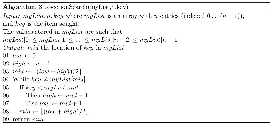
Simply stated the bisection search works as follows: Look at the element in the middle of the list and compare the key to the element in the middle position. If they are the same then the search is successful, otherwise we look next at either the bottom half of the list or the top half of the list depending on the result of the first comparison. We look at the bottom half if the key is less than the value in the middle of the list and we look at the top half of the list if the key is greater than the value in the middle of the list. This process is then repeated on the relevant half of the list. Each comparison halves the list being searched.
The algorithm for the bisection search is given in Algorithm 3. Note that this algorithm design technique of successively reducing the problem size until an answer can be computed directly can be considered as an example of decrease-and-conquer.
1.4.1 Correctness
Will this algorithm always give us the correct answer (the position of the key in the list) if it is given valid input? That is, if we try to search a sorted list of numbers for a number which is known to be in the list.
Theorem 3. Algorithm bisectionSearch will give the correct answer for any valid input. That is, it will return the position in the list of the value key.
Proof
For simplicity let us assume that \(key\) appears exactly once in the list (the proof would be very similar if this was not the case). Then what we are being asked to prove is that the algorithm will find \(key\) (and thus be able to return its position in the list). We will do this proof by contradiction.
Assume that bisectionSearch does not find \(key\) (that is, that \(key\) is in the list and the algorithm
never gets to it).
Recall that the input list is sorted in ascending order and the algorithm works by “throwing
away” parts of the list where key could not appear. The only way that the algorithm would
never reach \(key\) is if at some stage the algorithm was directed into a part of the list where \(key\)
could not appear. That is, if \(key\) was smaller than the value at \(mid\) but \(low\) was updated, or \(key\)
was larger than the value at \(mid\) but \(high\) was updated. Based on the rules of arithmetic this
would not happen. Thus eventually \(low = mid = high\) and \(key \neq myList[mid]\) would be False (in fact \(key = myList[mid]\)). This would contradict our assumption.
1.4.2 Complexity
Let us now see if our bisection search algorithm is an improvement on the linear search algorithm that we considered earlier. In doing our analysis it is reasonable (as before) to choose the basic operation of the algorithm as being a comparison of the key with a list element. Note, however, that in this algorithm the number of passes through the body of the \(while\) loop is directly related to the number of comparisons so determining the number of passes through the \(while\) loop will also give us a good indication of the work done by the algorithm.
Once again it should be clear that the algorithm will perform differently depending on where in the list of numbers the key appears.
1.4.2.1 Best case analysis
What is the best case for the bisection search? The best case performance of the bisection search algorithm is when the key is in the middle position of the array. In other words, when it is in the array position \(mid (= \lfloor(0 + (n − 1))/2 \rfloor)\). In this case, \(mid\) is calculated and the first test of the \(while\) loop condition will indicate that the key has been found. This is one basic operation and the algorithm is thus \(O(1)\) in the best case.
1.4.2.2 Worst case analysis
What is the worst case for the bisection search? This is a much harder question to answer and we will do so in the theorem given below.
Theorem 4. The bisection search algorithm works in \(O(\log_2 n)\) comparisons in the worst case.
Proof
To simplify the proof let us assume that \(n = 2^k − 1, k \geq 1\). Then it is sufficient to show that in the worst case at most \(k\) comparisons are required.
We will do this proof by induction.
Clearly if \(k = 1\) then the list only has one element in it (in position 0) because \(n = 2^1 − 1 = 1\) and this element is equal to \(key\) because we know that \(key\) must be in the list. Let us thus consider \(k = 2\) as our base case.
Base Case:
\(k = 2\) implies \(n = 2^2 − 1 = 3\). We have \(myList[0] < myList[1] < myList[2]\) (because we know the list must be in order). If the key is in \(myList[1]\) then \(mid = (0 + 2)/2 = 1\) and the key is found immediately — one comparison is made and the body of the \(while\) loop is not executed at all. This is the best case for a list of size 3.
The worst case is if the key is not in \(myList[1]\) but in \(myList[0]\) or \(myList[2]\). If the key is in \(myList[0]\) then \(key < myList[1]\) and the \(while\) loop is executed once, setting \(high = mid − 1 = 0\) which means \(mid = 0\) and the key is found after 1 execution of the \(while\) loop. This means that two comparisons of \(key\) with a list element are made. This is also true for the case that the \(key\) is in \(myList[2]\) (exercise left to dear reader).
Thus in the case \(k = 2\), 2 comparisons and 1 execution of the \(while\) loop are required in the worst case. This is the result we were looking for.
Induction Hypothesis:
Assume the theorem is true for \(k = m\) — that is, searching a list of length \(2^m − 1\) requires at most \(m\) comparisons (and \(m − 1\) executions of the \(while\) loop).
Inductive step:
We now want to prove that the result holds for \(k = m + 1\). The first calculation of \(mid\) gives \(mid = \lfloor (0 + ((2^{m+1} − 1) − 1))/2\rfloor = 2^m − 1\).
Thus the first comparison of \(key\) essentially leaves us with two lists of size \(2^m − 1\): the list from 0 to \(2^m − 2\) and the list from \(2^m\) to \(2^{m+1} − 1\). By the induction hypothesis searching each half list requires at most \(m\) comparisons. Thus there are at most \(m+1\) comparisons for \(k = m+1\).
We have thus shown that for any list of length \(n = 2^k − 1\), at most \(k\) comparisons are needed. Now \(2^k = (n + 1)\) ( as \(n = 2^k − 1\)) and so \(k = \log_2 (n + 1)\). Therefore \(g_W (n) = \log_2 (n + 1)\) is the complexity function for the worst case of this algorithm, so the algorithm is \(O(\log_2 n)\) in the worst case.
For values of \(n\) not of this form, we can apply the proof to \(n' = 2^k −1 = n+r, 0 \le r < n\). These \(r\) elements can be interpreted as a list of elements of maximum value appended to the original list.
The bisection search is very fast — 1 million entries are searched with at most 20 comparisons. For a million element list, a linear search requires on average half a million comparisons. Clearly the bisection search is more efficient but it requires a sorted list. The choice of which of these two approaches to use thus depends on the form of the list to be searched.
1.5 Bisection Search 2
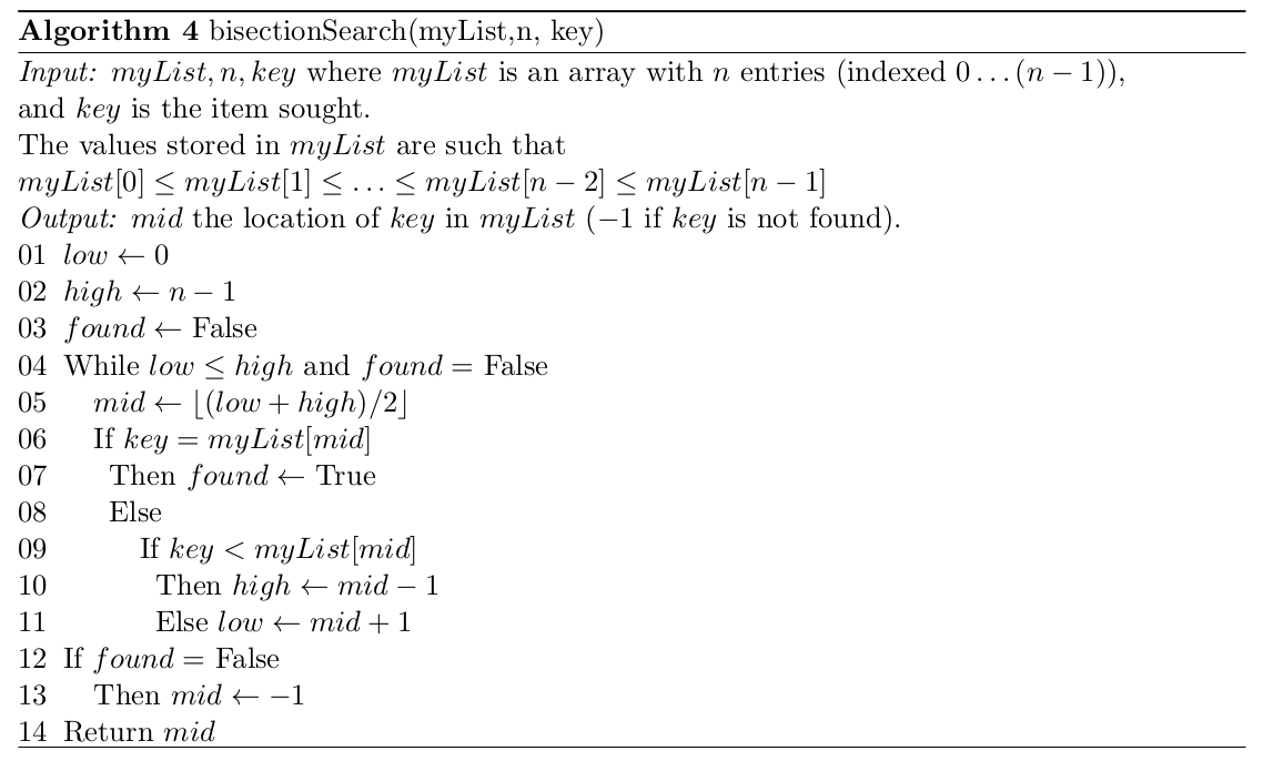
Suppose now that the key need not necessarily be in the sorted list of numbers which we are searching. Then our algorithm has to take this fact into account. If the number which is being searched for is not in the list then the process of searching the upper or lower part of the list after each comparison of the element in the middle position of the current sublist eventually leads to the situation where \(low > high\) and we have not yet found the key. The algorithm which deals with this case is given below.
1.5.1 Complexity
Note that the algorithm does two comparisons of the key against a list element inside the body of the loop. Note also that the number of such pairs of comparisons made by the algorithm is the same as the number of passes through the \(while\) loop. So we could consider the number of passes through the While loop as a good basic operation for the algorithm.
The best case for this algorithm is once again when the key appears in the middle position (\(\lfloor(low + high)/2\rfloor = \lfloor(0 + (n − 1))/2\rfloor = \lfloor(n − 1)/2\rfloor\)) of the original list. In this case the body of the \(while\) loop is executed once and one comparison is done. So the algorithm is in \(O(1)\) in the best case.
When does the worst case occur for this algorithm? Once again we can count the number of pairs of comparisons or the number of passes through the body of the \(while\) loop to get the complexity function \(g_W (n)\) of the algorithm. To get an idea of how much work the algorithm does in the worst case, suppose the algorithm is run on a list of length \(n > 1\). Here \(low \neq high\) and so the body of the loop is entered. Inside the loop a value for mid (\(\lfloor(low + high)/2\rfloor\)) is computed and \(key\) is compared with \(myList[mid]\).
In the worst case \(key \neq myList[mid]\) and so the algorithm adjusts either \(low\) or \(high\) to look in the appropriate sublist (numbers bigger than \(myList[mid]\) or numbers smaller than \(myList[mid]\)) on the next pass through the loop. There will be at most \(\lfloor n/2 \rfloor\) entries in the bigger of the two sublists (\(n/2\) if the original list was even and \((n/2) − 1\) if the list was odd). This means that the number of pairs of comparisons or passes through the \(while\) loop that the algorithm would do on the second pass (working on the smaller sublist) is at most the number of pairs of comparisons for searching a list of length \(\lfloor n/2 \rfloor\). This is \(g_W\) (\(\lfloor n/2 \rfloor\)).
This gives the recurrence relation \(g_W (n) = 1 + g_W (\lfloor n/2 \rfloor)\) which describes the performance of this algorithm in the worst case. In order to be able to solve this recurrence relation we need to establish a boundary condition — a point where we can directly calculate the value of \(W(n)\). Clearly if the original list is empty, of length 0, then no comparisons are done (the algorithm does not enter the loop as \(low > high\)) and so \(W (0) = 0\). It is, however, more useful to consider what happens for a list of length 1. Here \(low = high\) and so the body of the loop will be executed. In the body of the loop, \(key\) is compared with \(myList[0]\). If they are equal then \(found\) is changed to True and the loop would not be executed again. If they are not equal then either \(low\) or \(high\) is changed which would result in \(low\) being greater than \(high\) and the loop would not be executed.
So in both cases here, 1 pair of comparisons is made or the body of the loop is executed once. Thus if \(n = 1\) then \(g_W (n) = g_W (1) = 1\). (Note that we could get a list of length one in two ways –– if it is our original list in which case \(low = high = mid = 0\) or if we have arrived at a list of length 1 by successively shrinking our original list in which case \(low = mid = high\) but they do not necessarily point to position zero in the array.)
We thus have \(g_W(n) = 1 + g_W (\lfloor n/2 \rfloor)\) for \(n > 1\) and \(g_W(1) = 1\). Expanding the recurrence gives \(g_W (n) = 1 + g_W (\lfloor n/2 \rfloor) = 1 + 1 + g_W (\lfloor n/2^2 \rfloor) = 1 + 1 + 1 + g_W (\lfloor n/2^3 \rfloor)\) and so on. If the original list is of length \(n = 2^k\) then \(g_W (n) = \lg n + 1\). Each time the list is split a 1 is added to the sum on the right hand side of the equation and there can be at most \(\lg n\) such splits.
If the original list is of a more general form then we need to solve the recurrence relation (reduce the recurrence relation to its closed form, i.e. not referring to other values of \(g_W\)) by one or other of the standard techniques for doing so (see for example [Cormen et al., 1990], chapter 4 or [Brassard and Bratley, 1996], chapter 4). We can solve this recurrence relation by the method of “intelligent guesswork” –– expand the recurrence relation a few times, check for regularity, guess a suitable closed form and then prove this closed form is correct. In this case we have done the first two of these steps already and we know that the closed form should be something like \(\lg n\). Let us guess that \(g_W (n) = \lfloor \lg n \rfloor + 1\) and prove by induction that this result holds. Note that this choice seems sensible as lists of length \(n\) where \(2^k < n < 2^{k+1}\) seem to require one more pass through loop to find the key or determine that it is not there.
Theorem 5. \(g_W (n) = \lfloor \lg n \rfloor + 1\) for \(n \geq 1\)
Proof
Base case:
Let \(n = 1\). Then \(\lfloor \lg 1\rfloor + 1 = 0 + 1 = 1 = g_W (1)\) which is as we have seen before.
Induction hypothesis:
Let \(n > 1\) and assume that for \(1 \leq k < n, g_W (k) = \lfloor \lg k \rfloor + 1\).
Induction step:
\[\begin{align*} g_W (n) &= 1 + g_W (\lfloor n/2 \rfloor) \text{ by the recurrence relation} \\ &= 1 + \lfloor \lg \lfloor n/2 \rfloor \rfloor + 1 \text{ by induction hypothesis} \\ &= 2 + \lfloor \lg \lfloor n/2 \rfloor \rfloor \end{align*}\]
Now if \(n\) is even, then
\[ g_W(n) = 2 + \lfloor \lg n - 1 \rfloor = 1 + \lfloor \lg n \rfloor, \] since \(\lfloor n/2 \rfloor = n/2\) and \(\lg(n/2) = \lg(n) - \lg 2 = \lg n - 1\).
If \(n\) is odd, then
\[ g_W(n) = 2 + \lfloor \lg n - 1 \rfloor = 1 + \lfloor \lg(n-1) \rfloor = 1 + \lfloor \lg n \rfloor. \] This follows from the fact that \(\lfloor n/2 \rfloor = (n-1)/2\) and \(\lfloor \lg (n-1) \rfloor = \lfloor \lg n \rfloor\) when \(n\) is odd.
Thus, in all cases, \(g_W(n) = \lfloor \lg n \rfloor + 1\). Our binary search algorithm is thus \(O(\lg n)\) in the worst case.
The interested reader is referred to [Baase, 1988] for a treatment which proves that the Binary Search algorithm is also \(O(\lg n)\) in the average case.
1.5.2 Optimality
The next question we must ask about our bisection search algorithm is whether it is an optimal algorithm in the class of algorithms under consideration. Here we are dealing with searching algorithms which work by doing comparisons on list elements. In order to be able to answer the question of whether binary search is optimal we need to establish a lower bound on the number of such comparisons which are required. We will find this lower bound by means of a decision tree. Note that this optimality analysis is adapted from [Baase, 1988].
Let \(A\) be any algorithm in the class under consideration. We construct a decision tree for \(A\) and a list of size \(n\) by building a binary tree whose nodes are labelled with the numbers from \(0\) to \((n − 1)\) representing the indices of the list and whose nodes are arranged as follows. If \(j\) is the index of the first list element which the algorithm compares against the key, then we label the root of the tree with \(j\). Then for the remaining nodes (working from the root down), if a node is labeled \(i\), then we label the left child of \(i\) with the index of the list entry that the algorithm will compare \(key\) to if \(key < List[i]\) and we label the right child of \(i\) with the index of the list entry that the algorithm will compare \(key\) to if \(key > List[i]\). \(i\) will not have a left child if the algorithm halts after comparing \(key\) to \(List[i]\) and finding that \(key < List[i]\). Similarly for the right child. A leaf node would then indicate that the algorithm has not found the key but no further comparisons are made as the key cannot be in the ordered list.
Note that we could construct such a decision tree using the same procedure for any algorithm to find a given number in a list of numbers.
For a given input and a given value of key, the algorithm \(A\) would follow a path through the tree which is defined by making the appropriate comparisons and moving left or right depending on the result of each comparison. If at any stage \(key = List[i]\), then the path from the root would end in the node with label \(i\). If \(key \neq List[i]\) for any \(i\), then a leaf in the decision tree will eventually be reached. The number of comparisons made in the worst case by algorithm \(A\) is the number of nodes on the longest path from the root to a leaf in the tree. That is the height of the tree plus one, i.e. \(h + 1\). So if we can find a lower bound for the height of the decision tree which we create for Algorithm \(A\) then we will have a lower bound on the number of comparisons needed in the worst case.
Let \(h\) be the height of the decision tree and let \(N\) be the number of nodes in the tree. We know that \(h \geq \lfloor \lg N \rfloor\) (this result can be proved by induction). We now need to determine the relationship between \(N\) and \(n\) (the size of the input). We claim that every index to an element in the list must appear in the tree at least once, i.e. \(N \geq n\). We can prove this claim by a simple proof by contradiction.
Assume that there is no node in the tree labeled \(i\) for some \(0 \leq i \leq (n − 1)\). This means that at no point in the algorithm is \(key\) compared with \(List[i]\). This means that we can create two input lists, \(List1\) and \(List2\), with \(List1[i] = key\) and \(List2[i] \neq key\) and where \(List1\) and \(List2\) are identical otherwise and \(key\) does not appear in any of the other list positions. Now as \(List1\) and \(List2\) are the same except for the \(i\)th position which is not considered by algorithm \(A\) anyway, the same result should be returned if \(A\) is run on the two lists. Algorithm \(A\) does not, however, give the correct result for \(List1\) and so it cannot be correct –– it does not solve the given problem for all input instances. This is a contradiction and so there must be a node labeled \(i\) in the tree and so there must be at least \(n\) nodes in the tree. This means that \(N \geq n\). So \(h \geq \lfloor \lg N \rfloor \geq \lfloor \lg n\rfloor\).
Now we showed earlier that in the worst case \(A\) makes at least \(h + 1\) comparisons and so must make at least \(\lfloor \lg n \rfloor + 1\) comparisons. Recall that \(A\) was a randomly chosen algorithm from the class of algorithms under consideration which means that any algorithm in the class must do at least \(\lfloor \lg n \rfloor + 1\) comparisons for some input. Or alternatively that there exists some input for each algorithm in the class which will force the algorithm to make at least \(\lfloor \lg n \rfloor + 1\) comparisons.
The binary search algorithm does \(\lfloor \lg n \rfloor + 1\) comparisons in the worst case. So here the lower bound of the problem and the worst case of the algorithm are equal. This means that binary search must be optimal.
1.6 References
[Baase, 1988] Baase, S. (1988). Computer Algorithms: Introduction to Design and Analysis. Addison Wesley, Reading, Massachusetts, second edition.
[Baase and van Gelder, 2000] Baase, S. and van Gelder, A. (2000). Computer Algorithms: In- troduction to Design and Analysis. Addison Wesley, Reading, Massachusetts, third edition.
[Brassard and Bratley, 1996] Brassard, G. and Bratley, P. (1996). Fundamentals of Algorith- mics. Prentice Hall, Englewood Cliffs, NJ.
[Cormen et al., 1990] Cormen, T. H., Leierson, C. E., and Rivest, R. L. (1990). Introduction to Algorithms. The MIT Press, Cambridge, Massachusetts. Sixteenth Printing, 1996.