Chapter 6 Hashing
Content in this chapter was originally prepared and edited by Prof Ian Sanders and Prof Hima Vadapalli.
In many algorithms we want to be able to store information, typically referenced by a key, in a way which aids very fast look up. We would typically call a data structure that allows efficient insertion, searching and deletion a dictionary, and you will have likely already encountered such structures (e.g. Java’s HashMap and HashSet, or C++’s unordered_map or unordered_set). The underlying, language-independent data structure that these are all built are is known as a hash table
6.1 Direct Addressing
Our aim is to build a data structure that will allow us to store a number of unique keys. These keys could be integers, strings, or some other kind of object. Let us first assume the most basic case, which is known as direct addressing.
Here, we assume that we know every possible key that could occur, and assign a unique array position to every possible key which might be used in our application. In each array position we would then either store the element itself or a pointer to an “object” external to the direct addressing table. In a situation like this searching, inserting and deleting can be done very quickly and easily. We simply go to the appropriate position in the array to perform the operation required. Direct addressing works well if the range of possible keys is quite small.
A problem with this approach is that the “key space” (the domain of possible keys) could be very large and typically only a very small percentage of the keys would actually be used. This would result in a lot of wasted space if we even had enough space available but it is most often simply not feasible to allocate that amount of space.
Hashing gives us means of accomplishing the desired quick look up but at the same time does not require the same amount of memory.
6.2 Introduction to Hashing
Typically in hashing we map some key from the key space onto an integer which is an index into a hash table that stores the information we are interested in. The mapping from the key is done using a hash function and the result of the mapping is called the hash code of the key. We also say that for some hash function \(h\), the key \(k\) hashes to slot \(h(k)\).
In any set of keys it is possible that the application of a given hash function to two different keys could result in the same hash code being computed (we try to store both keys into the same place in the array). This is called a collision. It is important to try to choose a hash function which makes it unlikely that such collisions occur, but we cannot normally guarantee that collisions cannot occur.
Let us now consider a small example of hashing to see how the approach works. Suppose that the key space is pets’ names and the hash table is of size \(9\) — that is, has indices from \(0\) to \(8\). Let us now choose the hash function, \[ h(name) = \sum\limits_{i=1}^{length(name)} value(name_i) \mod 9, \] where \(value\) refers to the position of the character in the alphabet (\(value(a) = 1\), \(value(b) = 2\), etc.). IIf the pets’ names that we are interested in are “spot,” “fred,” “mutt,” “jeff,” “pina,” “flopsy,” “becca” and “fido” and we apply our hash function then we see that
\[ h(spot) = (19 + 16 + 15 + 20) \mod 9 = 70 \mod 9 = 7 \\ h(fred) = (6 + 18 + 5 + 4) \mod 9 = 33 \mod 9 = 6 \\ h(mutt) = (19 + 16 + 15 + 20) \mod 9 = 74 \mod 9 = 2 \\ h(jeff) = (10 + 5 + 6 + 6) \mod 9 = 27 \mod 9 = 0 \\ h(pina) = (16 + 9 + 14 + 1) \mod 9 = 40 \mod 9 = 4 \\ h(flopsy) = (6 + 12 + 15 + 16 + 19 + 25) \mod 9 = 93 \mod 9 = 3 \\ h(becca) = (2 + 5 + 3 + 3 + 1) \mod 9 = 14 \mod 9 = 5 \\ h(fido) = (6 + 9 + 4 + 15) \mod 9 = 34 \mod 9 = 7. \\ \]
If these are placed into our hash table as below then we see that the entries are spread out over the table even though three of the names start with an “f.” Unfortunately (as sometimes happens) we have a collision — “spot” and “fido” hash to the same slot in the table.
| Hash Code | Key(s) |
|---|---|
| 0 | jeff |
| 1 | |
| 2 | mutt |
| 3 | flopsy |
| 4 | pina |
| 5 | becca |
| 6 | fred |
| 7 | spot, fido |
| 8 |
In designing a hash table we have to worry about two (somewhat independent) things — what is a good hash function, and how do we handle collisions?
A good hash function should spread the hash codes for the input keys over the range of available indices to give as few collisions as possible and is often dependent on the application which the hash table is being designed for.
There are two common ways of dealing with collisions
- closed address hashing also called chained hashing
- open address hashing
We discuss each of these below.
6.3 Closed Address Hashing
In closed address hashing, each position in the table is a pointer to the head of a linked list. Initially all the lists are empty, i.e. the pointer to the head of the list (which is stored in the hash table) is nil.
To insert a key into the hash table, we first calculate its hash code (using the hash function that we have decided on) to get the index into the hash table and then we insert a node representing the key at the front of the linked list in that position.
The cost of an insertion is thus clearly \(O(1)\) — the cost of computing the hash code (which can be done in constant time) plus the cost of doing an insertion at the head of the appropriate list.
The cost of searching and the cost of deletion in the best case are both \(O(1)\) — if the key being searched for (or to be deleted) is at the head of the linked list. For a search we just have to calculate the hash code and then access the first element in the linked list. For a deletion we calculate the hash code and then remove the first element in the linked list by making the pointer point to the second node in the linked list.
In the worst case searching and deletion are both dependent on the length of the list in the slot being considered.
If the hash table is being used to store \(n\) items in \(h\) linked lists, then the load factor of the table, typically denoted by \(\alpha\), is \(n/h\) and this is the average number of items in each linked list. If we have chosen a good hash function for our table then the actual number of items in each list will be very close to \(\alpha\).
To search for a key in the table or to retrieve a key from the table, we must first calculate its hash code and then search the appropriate linked list. If we have a good hash function then the average search cost is \(O(1 + \alpha)\). This remains the same if the key is in the hash table or not.
To see this, let us consider a search for a key which is not in the table. First let us assume that any key is equally likely to hash to any of the \(h\) slots (i.e. we have a good hash function). Then the average time for an unsuccessful search is the average time to search to the end of each of the \(h\) lists. The average length of the lists is \(\alpha\) so the cost to search to the end of a list is \(\alpha\) (we need to compare the key to \(\alpha\) positions in the linked list). The average time including calculating the hash code is thus \(O(1 + \alpha)\). If \(h\) is proportional to \(n\), this is about \(O(1)\). If the key is in the hash table, then a similar, but slightly more complicated argument, leads to a similar result. The average cost of a deletion is also O(1 + \(\alpha\)).
Clearly the worst case for both searching and deletion is if we have a poor hash function and all of the keys hash to the same slot and are thus stored in the same linked list. Then searching for (or deleting) the last item in the list is \(O(n)\).
In order to improve the search time in each slot of the hash table it seems that we could use balanced binary search trees instead of linked lists. This is generally not done in practice due to complications of coding etc. Instead we try to come up with good hash functions. In addition, if the load factor increases because we are attempting to store many more keys than the size of the hash table then we can perform an operation called “array doubling” which increases the size of the hash table by doubling the number of available slots and spreading those keys already in the hash table out over the full extent of the new table. We will revisit this idea as part of the Computer Science Honours Analysis of Algorithms course.
6.4 Open Address Hashing
In this approach to hashing, keys are actually stored in the slots in the hash table not in a linked list. Each slot holds a key or a nil. If a collision occurs (because another key which hashes to that position has already been stored), then alternative positions in the hash table are considered (probed) based on some pre-defined rules. This is called rehashing.
Open address hashing is generally less flexible than closed address hashing as the table can fill up and load factors of greater than \(1\) are not possible. It is, however, more space efficient as we do not have to create linked lists as well as set aside the space for the hash table.
The simplest rehashing is called linear probing. If there is a collision at position/index \(j\) then the function \(rehash(j) = (j + 1) \mod h\) is used to calculate the new hash code. Note this approach just keeps looking in the next table position (taking wraparound into consideration) until a vacant position is found.
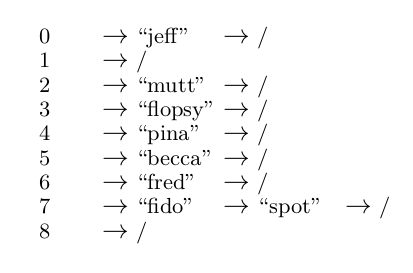
Recall that we had a collision in our previous example — “fido” hashed to the same slot as “spot.” If we used this simple approach to rehashing then “fido” would have been placed into the next slot. Our “rehashed” hash table would then have been as below.
| Hash Code | Key(s) |
|---|---|
| 0 | jeff |
| 1 | |
| 2 | mutt |
| 3 | flopsy |
| 4 | pina |
| 5 | becca |
| 6 | fred |
| 7 | spot |
| 8 | fido |
Searching/retrieval from an open address hash table is done by calculating the hash code and then searching in that position in the table. If the key is found then a successful search has been made. If there is a key in that position but it is not the key being searched for then rehashing is done and the next position in the rehashing sequence is checked. If the key is found or an empty slot is found then searching stops otherwise the process is repeated.
Clearly the best case for searching is \(O(1)\) — the hash code is calculated and the key is found in the first position searched (or that position is empty). Generally performance is good when searching a hash table with a low load factor. However, the average number of slots which have to be accessed approaches \(\sqrt{n}\) if the load factor is high i.e. close to \(1\).
We need to be careful when doing deletions from the hash table as we might be trying to delete a key which has caused a subsequent key to be rehashed to another slot in the table. We could lose track of which indices we have rehashed to and have the chain broken so that later searches would not complete successfully. One approach to dealing with this problem is to use an “obsolete” marker for deleted items. We would then know that at some time there had been a key stored in that slot and that we would have to rehash again to continue searching. Clearly if we were doing an insertion we could overwrite an “obsolete” marker with the key we are trying to store.
6.5 Hash Functions
As discussed above, the aim of a hash function is to spread the calculated hash codes uniformly over the range of indices available in the hash table — i.e. to accomplish simple uniform hashing. A common approach is to calculate some numeric value for the key, to optionally multiply this value by a constant, and then to take the remainder after dividing by the size of the hash table. The division method is thus \(h(k) = k \mod h\) or \(h(k) = Ak mod h\).
The multiplication method is a two step process – first we multiply the key \(k\) by a constant \(A\), \(0 < A < 1\) and extract the fractional part of \(kA\). Then we multiply this value by \(h\) and take the floor of the result \(h(k) = \lfloor h(Ak \mod 1) \rfloor\). Both of the approaches above can give poor performance on average for some keys.
Universal hashing attempts to “guarantee” good average case performance by selecting a hash function at random at run time from a carefully designed class of functions. More detail on hash functions can be found in the references below.
6.6 Summary Lecture
The video below summarises the content in this chapter. You may either watch it first, or read through the notes and watch it as a recap.
6.7 Additional Reading
- Introduction to Algorithms (Chapter 11), Cormen, Leisersin, Rivest and Stein, 3rd ed.
- https://programming.guide/hash-tables.html
- https://programming.guide/hash-tables-open-addressing.html