Chapter 2 Sorting
Content in this chapter was originally prepared and edited by Prof Ian Sanders and Prof Hima Vadapalli.
The video below summarises the content in this chapter. You may either watch it first, or read through the notes and watch it as a recap.
The next group of common algorithms which we will consider will be those for sorting. This is another task which is performed often when computers are used in industry so it is worthwhile understanding some of the classic approaches. We will not study all of the sorting algorithms which have been developed, merely an interesting subset of them.
These algorithms can be applied to sort data structures of various types. We will restrict our study to lists of numbers. In particular we will be trying to sort lists of numbers stored in arrays in memory.
2.1 Max Sort
Suppose that you were asked to sort a list of numbers. One way to tackle the problem would be to find the biggest number in the list and write that down, then to find the second biggest number in the list, then to find the third biggest number and so on.
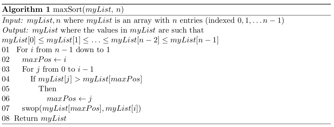
The max sort works in very much the same fashion. We start off by making a pass through the list to find which position in the list holds the biggest number. Then we swop the biggest number and the number in the last position. This means that the biggest number is now at the end of the list (the correct position for it to be if we are sorting from smallest to biggest). Then we look for the position of the biggest number in the list but now we do not consider the last position in the list. After this pass we swop this number (the second biggest number) with the number in the second last position in the original list. Having done this the last two numbers in the list are in sorted order. We then continue this process for all the numbers in the list.
The details of the max sort algorithm is given in Algorithm 1.
2.1.1 Correctness
Once again we should prove that the algorithm above will do what we want it to do if we supply it with valid input. That is if our input is a list of numbers then the algorithm will return the list of numbers sorted in ascending order (i.e. arranged from the smallest number to the biggest number). This can be done by a straightforward inductive proof.
Theorem 1. maxSort works correctly for any valid input.
Proof
Base case:
Let \(n = 2\). That is, let the length of the list be 2 (there are two numbers in the list – a list with only one number is already sorted). Then the outer loop will work from \(1\) down to \(1\). That is, it will execute exactly once.
In the body of the loop \(maxPos\) will be given the value of \(i\) which is \(1\) – it will point to array position 1 which holds the second number in the list. In the inner loop \(j\) goes from \(0\) to \(i − 1 = 1 − 1 = 0\) and so will also execute once. In the body of the inner loop, if \(myList[0] > myList[1]\) then \(maxPos\) is updated to point to position \(0\) in the array (the first number is bigger than the second number). If \(myList[0] \leq myList[1]\) then the first number is the smaller of the two and \(maxPos\) will not be changed. The inner loop will then be exited and the number in position \(1\) in the array will be swopped with the number in the position pointed to by \(maxPos\). If the numbers were originally sorted then the swop will change nothing – the number in position \(1\) in the array will be swopped with itself. If the numbers were not sorted then the numbers in positions \(0\) and \(1\) will be swopped. This list will now be sorted. The algorithm would then exit the outer loop and return the sorted list of numbers. The algorithm thus works for a list of length \(2\).
Induction hypothesis:
Assume now that the algorithm works for a list of length \(k − 1\) where \(k > 2\). This means that the algorithm will correctly sort a list of length \(k − 1\).
Inductive step:
We now need to show that the algorithm would work for a list of length \(k\). Consider what happens in the first pass through the outer loop. Here \(maxPos\) will be set to \(k − 1\) (to point to the last element in the list). The inner loop will then compare each of the numbers in positions \(0\) to \(k − 2\) to the number currently pointed at by \(maxPos\) and will update \(maxPos\) appropriately.
After the inner loop terminates \(maxPos\) will point to the biggest number in the list which will then be moved to the last position in the list. We thus have the biggest number in its correct position and a (possibly) unsorted list of length \(k−1\) in positions \(0\) to \(k−2\) of the array. By our induction hypothesis the algorithm will correctly sort a list of length \(k − 1\). This means that the algorithm will correctly sort the numbers in positions \(0\) to \(k − 2\) in the array (the first \(k − 1\) numbers in the list). The remaining passes through the outer loop accomplish this and so when the outer loop terminates the algorithm will return a correctly sorted list of numbers. So the algorithm will work correctly for a list of length k. Thus by the principle of mathematical induction our result is proved.
2.1.2 Complexity
Let us now analyse this algorithm. Clearly the algorithm has no best and worst case – for any list of length \(n\) it always does the same amount of work. To determine the amount of work the algorithm does we must first identify a basic operation which will give us a good idea of the amount of work done and then we must determine how many times this basic operation is executed. In this algorithm most of the work is done in comparisons between list elements so counting these comparisons is a good approximation to the amount of work that the algorithm does.
The algorithm has two loops. The outer loop controls the moving of the biggest number at each pass to the end of the list. The inner loop checks each number in the list being considered at any stage to determine if it is the biggest number in that sublist. In the first pass of the outer loop there are \(n\) numbers being considered so there are \(n − 1\) comparisons (the inner loop is executed \(n − 1\) times to compare each number in that sublist to the current maximum number).
In the next pass through the outer loop the sublist is of length \(n − 1\). The biggest number has been moved to the end of the list (the \(n − 1\)th position in the array) and we are only considering positions \(0\) to \(n − 2\) in the array with the \(n − 2\)th array element originally set as the maximum found so far. Thus there are \(n − 2\) comparisons. The next time round the sublist is of length \(n − 2\), then \(n − 3\), and finally of length 2. The total number of comparisons is thus \((n − 1) + (n − 2) + (n − 3) + \ldots + 2 + 1\). So the complexity function is \(g(n) = (n − 1) + (n − 2) + \ldots + 3 + 2 + 1 = n(n − 1)/2.\) The max sort algorithm is thus \(O(n^2)\).
2.1.3 Optimality
As we will see later the max sort algorithm is not an optimal algorithm. There are a number of more efficient sorting algorithms.
2.2 Selection Sort
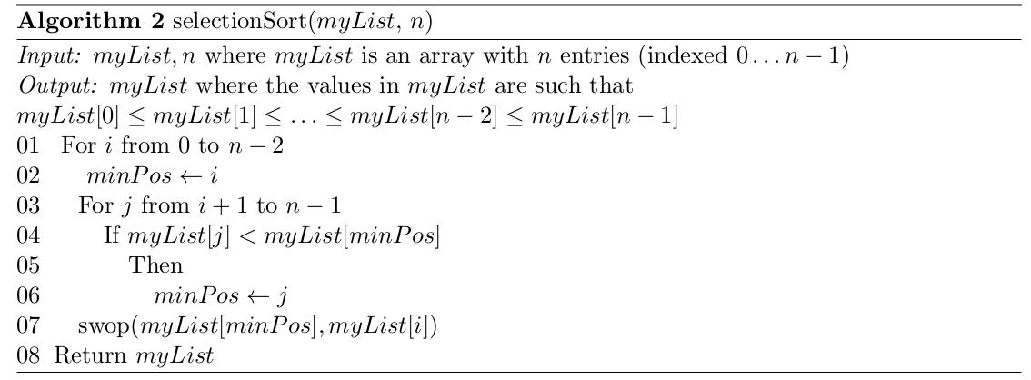
The Selection sort (also called the min sort) algorithm is very similar to the max sort algorithm except that in this case we move the smallest number into its correct position in the first pass of the algorithm, the second smallest number into its correct position in the second pass, and so on. The selection (or min) sort algorithm is shown in Algorithm 2.
The animation below shows the selection sort in action
Figure 2.1: On each iteration, the sort scans across the remaining part of the list to find a smaller number that the one under consideration. If it finds one, it then performs a swap. Then it moves on to the next number, until the list is sorted entirely. Animation from https://laptrinhx.com/selection-sort-in-javascript-1987349750/
The analysis for the selection sort is very similar to that for the max sort. The inner loop first does \(n − 1\) comparisons (comparing the numbers in positions \(1\) to \(n − 1\)), then \(n − 2\) comparisons, and so on. So once again the complexity function \(g(n) = n(n − 1)/2\) and the algorithm is \(O(n^2)\).
The proof of correctness of the solution method is very similar to that for max sort and, like max sort, selection sort is not an optimal algorithm.
2.3 Bubblesort
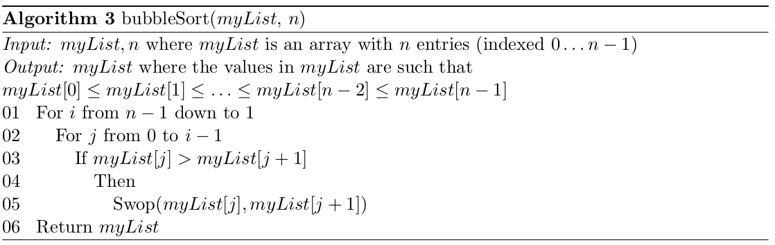
Another commonly used sorting algorithm is the bubble sort. This algorithm works by “bubbling” the largest number to the end of the list. Then “bubbling” the second largest number to the second last position in the list. Then the third largest number to the third last position and so on until the list is sorted. The algorithm works by comparing numbers which are next to each other in the list of numbers and interchanging the values if the first value is bigger than the second.
The animation below shows the bubblesort in action
Figure 2.2: Animation from https://medium.com/@dfellows12/comparing-bubble-selection-and-insertion-sort-89cf3b3dd8eb
This algorithm does the job it is required to do but how efficient is it? In order to answer this question, let us look at the work that the algorithm does and once again to do this we choose the basic operation as a comparison of two list elements.
The comparisons are made in the inner loop of the algorithm and there is one comparison each time the inner loop is executed. Thus counting the number of times the inner loop is executed will tell us how many comparisons are made. For a problem of size \(n\), the inner loop is executed first \(n − 1\) times, then \(n − 2\) times, …, and finally once only.
This means that in total the inner-loop is executed \(n(n − 1)/2\) times. This is \(O(n^2)\). This also means that the algorithm is \(O(n^2)\) in the number of comparisons of list elements made. This analysis gives us a measure of the efficiency of the bubble sort. (Most of the work is done in the inner-loop).
Exercise: Prove the bubble sort is \(O(n^2)\).
Is this a good measure of the amount of work the algorithm has to do? What would the complexity of the algorithm be if we chose the number of swops as the basic operation which we count to determine the complexity function of the algorithm? In this case the algorithm would display best and worst case performance. In the best case no swops would ever be done but we would still do \(O(n^2)\) comparisons – this would happen if every pair of numbers which was tested was already “in order.” This could only happen if the original list was already sorted.
In the worst case a swop would occur for every comparison. This would be the case if the original list was arranged in reverse sorted order (from biggest to smallest). The algorithm would then do \(n − 1\) swops to move the largest number from the beginning of the list to the end of the list. Then it would do \(n − 2\) swops to move the second largest number from the first position to the second last position in the list. And so on until the list is sorted. So the complexity function would be \(g(n) = n(n − 1)/2\) and the algorithm is \(O(n^2)\) in the worst case.
This raises the question of whether we can improve the bubble sort in any way so that it has an improved best case performance. One way to do this is to break out of the algorithm if on any pass of the inner loop no swops are made. If no swops are made then the list must be in order. The algorithm in Algorithm 4 works in this way.
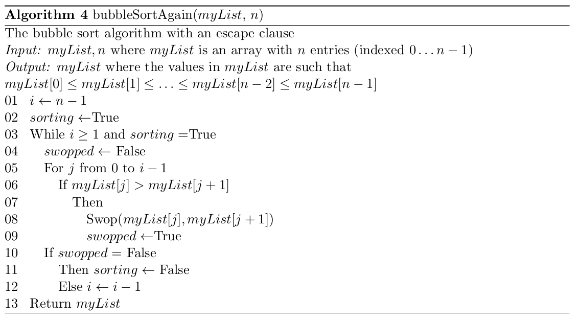
So if on any pass of the list, no swops are made then the algorithm breaks out of the outer loop and terminates. The algorithm will however always have to make at least one pass through the inner loop in order to check if any swops are made. The algorithm will thus do at least \(n − 1\) comparisons of list elements. The best case for this version of bubble sort is thus \(O(n)\) and the worst case remains as \(O(n^2)\).
The bubble sort is simple but not very efficient. If one was sorting to be able to use the results of the sort later or if it was a one-off job, then it might be OK, but there are better algorithms for sorting and we will be looking at some of these in the next sections of this chapter.
2.4 Insertion Sort
The next sort we will consider is the insertion sort. This sort works by maintaining a sorted sublist of numbers and inserting the next number into the correct position of the sorted sublist which then becomes one number longer. The process is then repeated for the next number.
The algorithm starts by treating the first number in the list as the sorted sublist and the inserting the second number into the appropriate position in the sublist — before the first number if it is smaller than the first number and after it otherwise (remember we are dealing with distinct numbers, so the two numbers cannot have the same value). Note if the second number is smaller than the first, then the first number has to be shifted from position 0 in the array into position 1 so that the second number can be slotted into position 0. If the second number is bigger than the number in the sorted sublist then the length of the sorted sublist is increased.
The third number in the original list is handled in a similar fashion. First it is compared to the second number in the sorted sublist. If it is bigger then the sorted sublist is increased in length by 1. If it is smaller then it is compared to the first number in the sorted sublist. If it is bigger than the first number it is slotted in between the first and second numbers by moving the second number one space to the right and putting the new number into the position which has been “opened up” in the sorted sublist. If the number we are inserting is smaller than the first number in the list then it must be inserted at the beginning of the list. This means that all of the numbers have to be shifted along to make room. First the second number in the sorted list is shifted one place to the right (into the position which was occupied by the number we are inserting). Then the first number is shifted into the position freed up by the second number and then finally the number we are trying to place is inserted into the beginning of the sorted sublist (at position 0). This process is then repeated for all of the other numbers in the unsorted sublist.
This procedure is best illustrated in the animation below:
Figure 2.3: Animation on Insertion Sort from https://commons.wikimedia.org/wiki/File:Insertion-sort-example.gif
The insertion sort algorithm is shown in Algorithm 5.
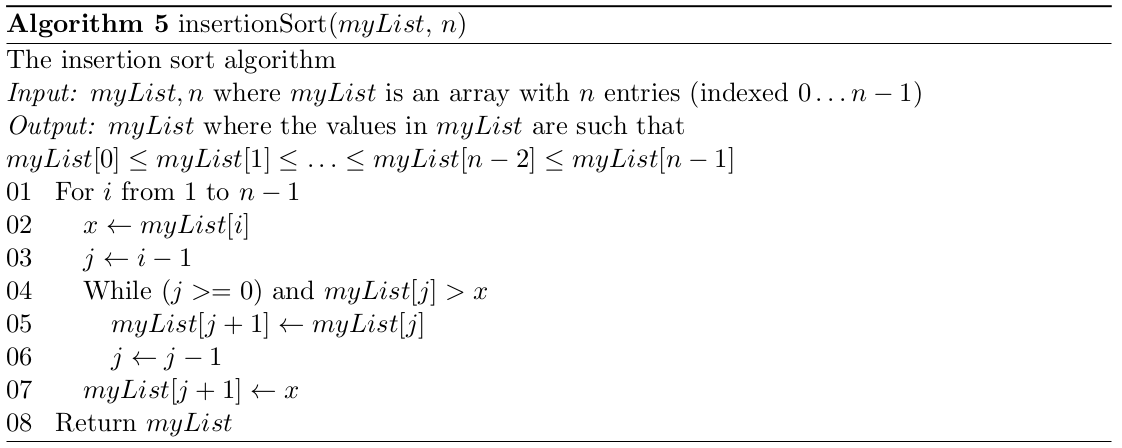
To analyse this algorithm we can once again consider the comparisons of two list elements as the basic operation. It should be easy to see that this algorithm performs different amounts of work on different inputs (i.e. it exhibits best and worst case behaviour).
When does the algorithm do the fewest comparisons? If the test \(myList[j] > x\) fails (i.e. \(myList[j] < x\) is true) then the algorithm will not enter the body of the loop and will then not test that condition again on any pass through the outer loop. So if on each pass of the outer loop, the test \(myList[j] > x\) fails immediately, then the least number of comparisons will be made.
What would the format of the input list have to be for this to occur? On each pass through the outer loop, \(x\) (the number we are trying to insert into its correct place) would have to be bigger than the biggest number in the sorted sublist. This would only occur if the original list was already in sorted order! In this case we would do one comparison of list elements for each pass of the outer loop so we would do \(n − 1\) such comparisons in total. Our insertion sort algorithm is thus \(O(n)\) in the best case.
Similarly the algorithm does the most work (the most comparisons of list elements) when the number which is being inserted into the sorted sublist is smaller than all of the numbers which are already in that sorted sublist. \(x\) is compared to the last number in the sublist, then to the second last, and so on until it is compared to the first number in the sublist.
When the sorted sublist has only one number in it then only one comparison is made, when it has two numbers then two comparisons are made, and so on. When the algorithm is trying to insert the last number into its correct place, the sorted sublist has \(n − 1\) numbers in it and so \(n − 1\) comparisons are made. Thus \(g_W(n) = 1+2+3 \ldots (n−2)+(n−1) = n(n−1)/2\) and so insertion sort is \(O(n^2)\) in the worst case.
What about the average case performance of insertion sort? To do the analysis, we assume that the numbers we are sorting are distinct and that all arrangements (permutations) of the elements are equally likely.
Let us now consider what will happen when we try to insert the \(i\)th number of the original list into its correct position in the ordered sublist, which is of length \(i − 1\). There are \(i\) places where this number could occur. It could be bigger than all the numbers, it could fit between the biggest and the second biggest number in the list, or between the second biggest and the third biggest number, and so on. It could also be smaller than the first number.
If the number is bigger than all the numbers in the sorted sublist, then it takes one comparison to establish this. If it is bigger than the second biggest number, but smaller than the biggest number, then two comparisons are required to establish this. And so on. If the number we are trying to insert into the list is smaller than all of the numbers in the sorted sublist except for the first number in the sorted sublist, then it takes \(i − 1\) comparisons to establish this. If the number we are trying to insert into the list is smaller than all of the numbers then we find this out when we compare it to the first number and so this case also takes \(i − 1\) comparisons. By our assumption all of the positions are equally likely so to the average number of comparisons to insert our number into a sorted sublist of length \(i\) is
\[ \sum\limits_{j=1}^{i-1} \dfrac{1}{i} \cdot j + \dfrac{1}{i} \cdot (i-1) = \dfrac{1}{i} \sum\limits_{j=1}^{i-1} (j) + 1 - \dfrac{1}{i} = \dfrac{i+1}{2} - \dfrac{1}{i} \]
If we now consider the comparisons required for inserting each number in the original list into the sorted sublist, then
\[ g_A(n) = \sum\limits_{i=2}^{n} (\dfrac{i+1}{2} - \dfrac{1}{i}) = \dfrac{n^2}{4} + \dfrac{3n}{4} - 1 - \sum\limits_{i=2}^{n} \dfrac{1}{i} \]
Now, \(\sum_{i=2}^n \dfrac{1}{i} \approx \ln(n)\) and therefore
\[ g_A(n) \approx \dfrac{n^2}{4} + \dfrac{3n}{4} - 1 - \ln(n) \]
and so \(g_A(n) \in \Theta(n^2)\).
Insertion sort is thus \(O(n)\) in the best case and \(O(n^2)\) in the average and worst cases. In practice, insertion sort works quite efficiently. We will, however, study some more efficient algorithms later in the text. The fact that there are more efficient sorting algorithms (that also work by comparisons of list elements) means that insertion sort (and max sort, selection sort and bubblesort) is not optimal.
Once again a simple inductive proof can be used to show that the insertion sort algorithm is correct, but we will leave this as an exercise to the reader.
2.5 Mergesort
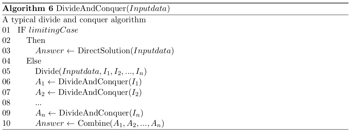
The next algorithm we will look at is a member of the class of divide-and-conquer solutions. Typically divide-and-conquer solutions to problems are based on the approach of dividing the original problem instance into two (or more) roughly equal smaller parts, solving the smaller instances recursively (i.e. in the same manner by once again dividing them into smaller instances) until a limiting case is reached which can be solved directly and then combining the solutions to produce the solution to the original problem. A skeleton of a typical divide and conquer algorithm is given in Algorithm 6.
The mergesort algorithm is a typical divide and conquer algorithm, a simple skeleton of which is shown in Algorithm 7. This algorithm works on a list of numbers stored in an array in memory. The parameters \(left\) and \(right\) are the positions of the first element and last element in the array to be sorted. Initially, \(left\) would be \(0\) and right would be \(n − 1\), where \(n\) is the length of the list being sorted.
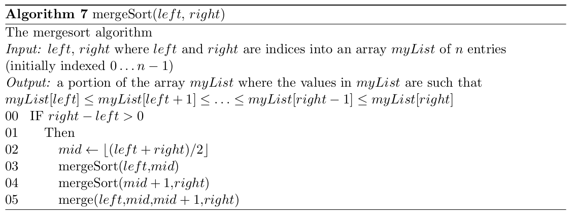
This algorithm is clearly recursive (there are two calls inside the body of the algorithm to the
algorithm) — it divides the current list in half at each level of recursion and then calls mergesort
to sort the halves of the list. The merge, which reassembles the sorted list from the two sorted
half lists, must still be specified properly.
We will look now at a more complete specification of mergesort, which works by successively
dividing the list into smaller and smaller lists until the limiting case of a one element list is
reached. Once the limiting case of the recursion has been reached the algorithm begins “bubbling out” merging the sorted half lists at each level of recursion.
To accomplish the merging of the two sorted half lists at each level we need a second array. This array stores the unmerged half lists in a back to back fashion with the right half list in reverse order. This temporary list is then used to merge the two half lists back into the original list by looking at the ends of the list, and copying the smallest element into the first position of the original list, shrinking the temporary list appropriately and continuing until all the values have been copied into the original list in sorted order.
The full mergesort algorithm can then be written out as in Algorithm 8.

This procedure is illustrated in the animation below:

Figure 2.4: Animation on mergesort from https://upload.wikimedia.org/wikipedia/commons/c/cc/Merge-sort-example-300px.gif
Theorem 2. mergesort requires about \(n \lg n\) comparisons to sort a list of \(n\) elements.
Proof
For mergesort, we have an algorithm that has to make a linear pass (the merging phase) through
the data after it has split and sorted the two halves. The splitting of the list can be done in
constant time. Sorting each half list takes half as much time as sorting the whole list and sorting
a list of length 1 takes no work.
So we can derive the reccurence relationship
\[ g(n) = g(\lfloor \dfrac{n}{2} \rfloor) + g(\lceil \dfrac{n}{2} \rceil) + n \text{ and } g(1) = 0, \] which describes the amount of work done by the algorithm for \(n\) elements of input.
Now if we consider a list of size \(n = 2^m\) we get
\[ g(n) = 2 g( n/2 ) + n = g(2^m ) = 2 g(2^{m−1}) + 2^m. \]
If we now divide through by \(2^m\) we get
\[ \dfrac{g(2^m)}{2^m} = \dfrac{g(2^{m-1})}{2^{m-1}} + 1. \]
Substituting for \(\dfrac{g(2^{m-1})}{2^{m-1}}\) in this formula gives
\[ \dfrac{g(2^m)}{2^m} = \dfrac{g(2^{m-2})}{2^{m-2}} + 1 + 1. \]
If we continue making these recursive substitutions, we will eventually converge at
\[ \dfrac{g(2^m)}{2^m} = m \Rightarrow g(2^m) = m \cdot 2^m. \]
But we have that \(n = 2^m\) and therefore
\[ g(n) = n \lg n. \]
The relationship clearly applies if \(n=2^m\), but it turns out that it also holds even when this is not the case (we will not do the analysis here). Therefore, mergesort is \(\Theta(n \lg n)\)
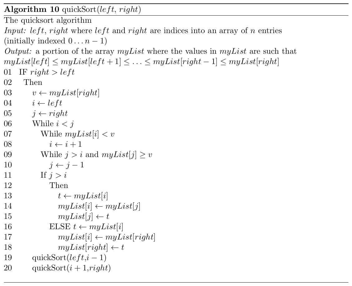
2.6 Quicksort
Quicksort is another “divide-and-conquer” method for sorting. It works by partitioning the list into two parts and then sorting the parts independently. The position of the partition depends on the list being sorted. An skeleton algorithm for the quicksort (again working on an array in memory) is thus as shown in Algorithm 9.
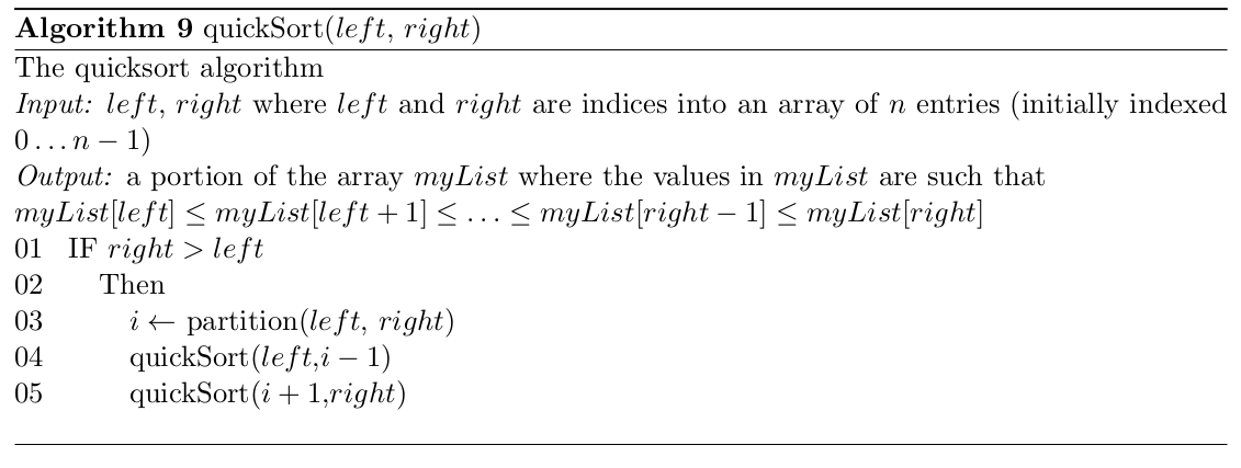
The crux of the algorithm is the partition.
The partition must rearrange the list to make the following 3 conditions hold:
- the element \(myList[i]\) is in its final place in the list for some \(i\)
- all the elements in \(myList[left] \ldots myList[i − 1]\) are less than or equal to \(myList[i]\).
- all the elements in \(myList[i + 1] \ldots myList[right]\) are greater than or equal to \(myList[i]\).
How is this done in practice?
- Choose \(myList[right]\) as the element to go to the correct place in the list.
- Scan from the left until an element \(\ge myList[right]\) is found.
- Scan from the right until an element \(< myList[right]\) is found.
- Swap these elements.
- Continue this way until the scan pointers cross.
- Exchange \(myList[right]\) with the element in the leftmost position of the right sub list (i.e. the element pointed to by the left pointer).
The complete quicksort is thus as shown in Algorithm 10.
Let us now consider the complexity of the quicksort algorithm. The best thing that could happen in quicksort would be that each partitioning divides the list exactly in half. This would mean the number of comparisons would satisfy the divide-and-conquer recurrence \(g(n) = 2 g( n/2 ) + n\) and \(g(1) = 0\).
The \(2g(n/2)\) is the cost for sorting the two half lists and the \(n\) is the number of comparisons at each level. We have already seen that \(g(n) = n \lg n\). That is, the best case for the quicksort is \(O(n \lg n)\). We can prove (but won’t do it here) that the average case for the quicksort is \(2n \ln n\) or \(O(n ln n)\).
Let us now consider the worst case of the quicksort algorithm. First notice that at any level of
the recursion, the partition will make \(k − 1\) comparisons of the partition element \(v\) with list
elements for a list of length \(k\). Once these comparisons have been made, the partition element
is moved into its correct place in the list for that level. If the partition element is the biggest
number in the list, then all that happens is that the list of length \(k\) is split into a list of length
\(k − 1\) and a list of length \(0\) on opposite sides of the partition element.
At the next level of recursion, for the list of length \(k −1\), \(k −2\) comparisons would be done to find to correct place for the partition element. If the partition element was again the biggest element in the list, then we would again get a bad partition — into a list of length \(k−2\) and a list of length \(0\).
For any list of length \(n\), the situation of the partition element always being the biggest element in the sublist being considered would occur if the list was already sorted before the quick- sort algorithm was called. In this case \((n − 1) + (n − 2) + (n − 3) + \ldots + 2 + 1\) comparisons would be made. This means that \(n(n − 1)/2\) comparisons of list elements would be done in total. The worst case of quicksort, when the list is already sorted, is thus \(O(n^2)\).
Note that there are a number of different ways of performing the partition in the quicksort algorithm, but they all give the same analysis.
2.7 Optimal Sorting
We will not consider the optimality of these algorithms in any detail in this course –– the proofs are quite difficult and we don’t have the time to go into them. However, we discussed some intuition in one of the videos why the lower bound for sorting algorithms which work by comparisons of list elements (as these do) is approximately \(n \lg n\).
This means that mergesort can be considered as an optimal sorting algorithm in this class of problem. Max sort, selection sort, bubblesort and insertion sort are obviously not optimal.
There are other sorting algorithms based on other approaches which work in linear time, such as counting sort, but we will not cover them here.
Finally, an obvious question to ask is which sort we should use in practice. It turns out that there’s no simple solution, but the default implementations of most programming languages usually implement their sorts using a hybrid approach — that is, they swap algorithms depending on the size and form of the data. For example, a simple hybrid approach would be to employ mergesort, but when the length of the sublist becomes less than some threshold, switch over to insertion sort just for that portion of the sort.
C++ uses Introsort, which is a combination of quicksort, heapsort (a sort we did not cover here) and insertion sort. More modern languages such as Python use an extremely optimised and complex sorting algorithm known as Timsort, which has optimal theoretical bounds, but is also optimised to work extremely well on real world data. Interested readers are encouraged to look these up online.
2.8 References
For a comparison of different sorts, please see https://www.toptal.com/developers/sorting-algorithms and https://www.cs.usfca.edu/~galles/visualization/ComparisonSort.html:
[Baase, 1988] Baase, S. (1988). Computer Algorithms: Introduction to Design and Analysis. Addison Wesley, Reading, Massachusetts, second edition.
[Baase and van Gelder, 2000] Baase, S. and van Gelder, A. (2000). Computer Algorithms: In- troduction to Design and Analysis. Addison Wesley, Reading, Massachusetts, third edition.
[Brassard and Bratley, 1996] Brassard, G. and Bratley, P. (1996). Fundamentals of Algorith- mics. Prentice Hall, Englewood Cliffs, NJ.
[Cormen et al., 1990] Cormen, T. H., Leierson, C. E., and Rivest, R. L. (1990). Introduction to Algorithms. The MIT Press, Cambridge, Massachusetts. Sixteenth Printing, 1996.