Chapter 4 Dynamic Programming
Content in this chapter was originally prepared and edited by Prof Ian Sanders and Prof Hima Vadapalli.
4.1 Shortest Path Problem
In the last section of the course we considered greedy algorithms and saw that there were some problems which could not be solved using a greedy approach. Let us consider the following shortest path problem: Given a weighted directed acyclic graph and a pair of nodes in the graph, find a shortest path from the start node, \(v_s\) , to the destination node, \(v_e\).
Example: In the graph below find the shortest path from \(v_1\) to \(v_2\).
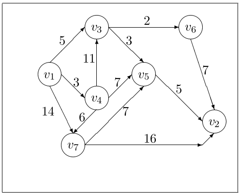
The obvious greedy approach for solving this problem –– repeatedly adding the shortest path from the city reached so far to any city which has not yet been visited –– does not always give the shortest distance. Consider trying to find the shortest distance between \(v_1\) and \(v_2\) using this greedy approach.
The first edge picked at \(v_1\) would be that leading to \(v_4\) which has a weight of \(3\). This is actually a bad choice in the global sense. The greedy approach would lead to a path of \(v_1\) , \(v_4\) , \(v_7\) , \(v_5\) , \(v_2\) for a distance of \(21\). The actual shortest path is \(v_1\) , \(v_3\) , \(v_5\) , \(v_2\) for a distance of \(13\).
We can, however, still solve this problem without having to test every possible route from \(v_1\) to \(v_2\) explicitly. First notice that \(v_1\) is adjacent to three other cities (vertices). The minimum distance from \(v_1\) to \(v_2\) is thus the smallest of the distances from \(v_1\) to each of those cities plus the shortest distance from that city to \(v_2\) . If \(D(v_k)\) is used to indicate the shortest distance from city \(v_k\) to \(v_2\) then we have that
\[ D(v_1) = \min(5 + D(v_3), 3 + D(v_4), 14 + D(v_7)) \]
So we are solving this problem by first solving three smaller problems of the same type and then “combining” the solutions from those problems to get the solution to our original problem. Thus this problem exhibits the “optimal subproblem property,” referred to in the Section on Greedy Algorithms.
Finding \(D(v_3)\), \(D(v_4)\) and \(D(v_7)\) is done in the same way. For example,
\[ D(v_4) = \min(11 + D(v_3), 7 + D(v_5), 6 + D(v_7)) \]
Note that breaking down the problem like this implies a recursive solution, However, as we can see (even in our simple example) such a recursive approach would lead to recalculation of some distances. Here \(D(v_3)\) would be calculated in determining \(D(v_4)\) as well as \(D(v_1)\). A better (more efficient) way of dealing with this problem is to use dynamic programming and to attack it in a “bottom up” style. In this case starting from the destination city, \(v_2\) , and working back to \(v_1\).
In our example, \(v_5\) and \(v_6\) only lead to our destination city, \(v_2\), so we start our calculation there — \(D(v_5) = 5\) and \(D(v_6) = 7\). Next we consider those cities which lead only to the cities in our “terminal cities” set — now \(\{v_2 , v_5 , v_6 \}\). Here we would consider \(v_3\) and \(v_7\). Now \(D(v_3) = \min(3 + D(v_5), 2 + D(v_6))\). \(D(v_7)\) is slightly different as \(v_7\) is connected directly to \(v_2\) . Thus \(D(v_7) = \min(7 + D(v_5 ), 16 + D(v_2))\) (where we know that \(D(v_2) = 0\)). We now add \(v_3\) and \(v_7\) to our set of terminal cities as we know the shortest distance from each of them to the destination city \(v_2\).
We would then apply the same process with \(v_4\) — it is the only city which we have not yet considered which has paths to only cities in our terminal cities set. Once we have calculated \(D(v_4)\) we could then calculate \(D(v_1)\).
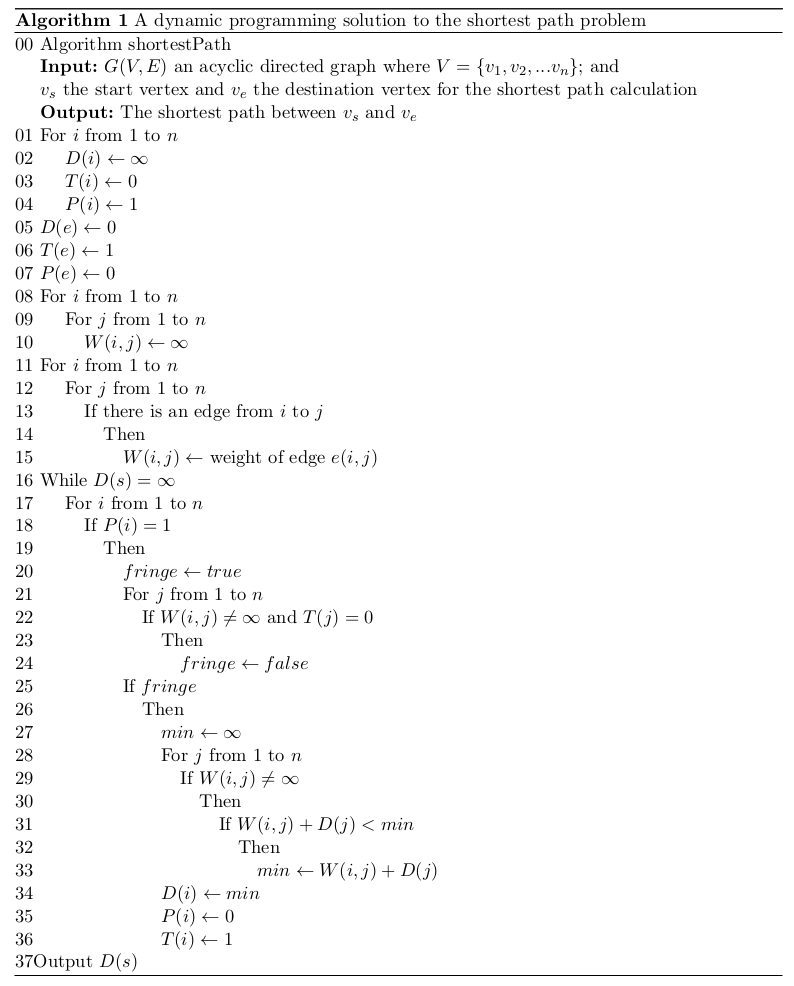
An algorithm to solve this problem is shown in Algorithm 1. The data structures used in this algorithm are an array \(D\) to store the distance of the shortest path from each vertex to the destination vertex and an adjacency matrix \(W\) which stores the distance between two vertices which are adjacent. Initially all the values in \(D\) would be set to \(\infty\) (or some undefined value) and then the value for the destination vertex would be set to \(0\). In the example we are considering \(D\) would initially be
\[ \begin{pmatrix} \infty \\ 0 \\ \infty \\ \infty \\ \infty \\ \infty \\ \infty \end{pmatrix} \]
and \(W\) would be
\[ \begin{pmatrix} \infty & \infty & 5 & 3 & \infty & \infty & 14 \\ \infty & \infty & \infty & \infty & \infty & \infty & \infty \\ \infty & \infty & \infty & \infty & 3 & 2 & \infty \\ \infty & \infty & 11 & \infty & 7 & \infty & 6 \\ \infty & 5 & \infty & \infty & \infty & \infty & \infty \\ \infty & 7 & \infty & \infty & \infty & \infty & \infty \\ \infty & 16 & \infty & \infty & 7 & \infty & \infty \end{pmatrix} \]
Note that the algorithm also uses two other arrays. \(P\) to indicate vertices/cities which are still to be considered and \(T\) to indicate vertices which are in the terminal set (i.e. we have already calculated the shortest distance from each of these vertices to the destination).
4.1.1 Complexity
Let us now consider the complexity of our dynamic programming solution. Initialising the arrays \(D\), \(P\) and \(T\) takes \(O(n)\) time and initialising the matrix \(W\) takes \(O(n^2)\) time. So overall initialisation is \(O(n^2)\) time.
Let us now consider the portion of the algorithm which actually calculates the shortest path (lines 16 to 36). Note that each path through the while loop that starts at line 16 results in at least one value in \(D\) being calculated (i.e. an \(\infty\) being replaced by a calculated distance to the destination). There are thus at most \(n − 1\) passes through the While loop. On each pass through the While loop we consider every vertex but actually only do work for those vertices which are not already in the terminal set by that pass. Here we first determine if the vertex is on the “fringe” (i.e. it is connected only to vertices in the terminal set) (lines 20 to 24) and then, if it is on the fringe, determine the distance from it to the destination vertex using the distances that have already been calculated in earlier passes. Both of these tasks are \(O(n)\). This means that each pass through the For loop (starting at line 17) does \(O(n)\) work and there are \(n\) passes through the loop for a total of \(O(n^2)\) work. The For loop is embedded in the While loop so in the worst case this algorithm takes \(O(n^3)\) time overall.
4.1.2 Correctness
Finally we need to convince ourselves that our algorithm will always return the shortest distance from the source vertex to the destination vertex. We can do this by means of an induction-like proof. Clearly the distance from the destination vertex, \(v_e\) , to itself must be 0 so setting \(D(e) \gets 0\) is correct.
In the first pass through the While loop only those vertices which are connected directly to the destination vertex are considered. There can be exactly one path from each of these vertices to the destination vertex (the edge that connects them) so the algorithm will correctly set the shortest path from each of these vertices to the destination vertex. This is the base case for our inductive proof.
Let us now assume that we have reached the stage of our algorithm where we have added a number of vertices to the terminal set and for each of these vertices we have correctly calculated the shortest path to \(v_e\) (our induction hypothesis). On the next pass through the While loop we consider in turn each vertex, say \(v_i\) , that has not yet been dealt with. First we determine if this vertex is only connected to vertices in the terminal set. This is done in lines 20 to 24 and is accomplished by checking whether each vertex which the current one is connected to is in \(T\) — it would be in \(T\) if \(T(j) = 1\). If any \(T(j) = 0\) then that vertex, \(j\), is not in the terminal set and thus the current vertex will not be considered further. If the current vertex is connected only to vertices in the terminal set then we determine the distance to \(v_e\) through each of these by using the edge connecting them and the previously calculated shortest path from each of those vertices to \(v_e\) . We then pick the shortest of these distances and make that the shortest path from \(v_i\) to \(v_e\) . We then add \(v_i\) to the terminal set. Clearly this will give us the shortest distance from \(v_i\) to \(v_e\) : There is only one direct path from \(v_i\) to each of its neighbours in \(T\) so we get the shortest distance there. By our induction hypothesis we have the shortest path from each of the neighbours in \(T\) to \(v_e\) . And we pick the shortest of the new distances and make this the shortest path from \(v_i\) to \(v_e\).
This means that our algorithm will always find the shortest path from some vertex, \(v_i\) , to \(v_e\) and so will eventually find the shortest path from \(v_s\) to \(v_e\) . The solution method is correct.
4.2 Properties of Dynamic Programming
The above algorithm has a number of features which are common in dynamic programming. First the approach used to tackle the problem seems to be a recursive solution but one where we might repeatedly calculate the solutions to some problems. To avoid doing this we work bottom up — building the solution to the original problem up from solutions to smaller subproblems. Next we see that we use various “tables” to store the information about the subproblems for use in solving the original problem. In this case we use the array \(D\) as our main table plus the arrays \(T\) and \(P\) to store some subsidiary information (and \(W\) is used to store the original input information).
Dynamic programming can be used when a problem exhibits two characteristics: optimal substructure and overlapping subproblems. The optimal substructure problem is the same as that in the previous chapter: Can the solution to the problem we care about be obtained from solutions to subproblems?. The notion of overlapping subproblems is what distinguishes dynamic programming from other approaches. For instance, if subproblems do not overlap, then a recursive solution is sufficient (e.g. binary search). However, when we need to potentially use the solution to a single subproblem multiple times, we can save time by recording its result the first time, and using that result every subsequent time.
There are two equivalent ways to implement dynamic programming, which we will illustrate with the following problem.
Example: The Fibonacci Series is a sequence of integers where the next integer in the series is the sum of the previous two. The sequence is defined by the following recursive formula: \(F(0) = 0, F(1) = 1, F(N) = F(N-1) + F(N-2)\). Calculate the \(N\)th Fibonacci number.
A recursive, non-dynamic programming approach looks like this:
#include <iostream>

using namespace std;

int fibonacci(int N){

  if (N == 0 || N == 1){
    return N;
  }
  return fibonacci(N-1) + fibonacci(N-2)
}

int main(){
  int N;
  cin >> N;
  cout << fibonacci(N) << endl;
}
The first approach is top-down with memoization. Here, we write the procedure in its natural recursive form, but modify it to save the results of each subproblem in a table or data structure. Then, before we solve a subproblem, we first check that we have not already solved it! Attacking the Fibonacci problem in a top-down manner looks like this:
#include <iostream>

using namespace std;

int fibonacci(int N, vector<int>& memo){
  if (N == 0 || N == 1){
    return N;
  }
  if (memo[N] != -1){
    return memo[N];  //we've compute the answer already
  }
  // compute answer and store it
  memo[N] = fibonacci(N-1, array) + fibonacci(N-2, array)
  return memo[N];
}

int main(){
  int N;
  cin >> N;
  vector<int> memo(N + 1, -1); // set all to -1 (unseen)
  cout << fibonacci(N, memo) << endl;
}
The second approach is the bottom-up method. This approach typically depends on some natural notion of the “size” of a subproblem, such that solving any particular subproblem depends only on solving “smaller” subproblems. We sort the subproblems by size and solve them in size order, smallest first. When solving a particular subproblem, we have already solved all of the smaller subproblems its solution depends upon, and we have saved their solutions. We solve each sub- problem only once, and when we first see it, we have already solved all of its prerequisite subproblems. Tackling the Fibonacci problem bottom-up looks like this:
#include <iostream>

using namespace std;

int fibonacci(int N){
  if (N == 0 || N == 1){
    return N;
  }
  int a = 0;
  int b = 1;
  for (int i = 2; i <= N; ++i){
    int temp = a + b;
    a = b;
    b = temp;
  }
  return b;
}

int main(){
  int N;
  cin >> N;
  cout << fibonacci(N) << endl;
}
In general, these two approaches yield algorithms with the same asymptotic running time, except in unusual circumstances where the top-down approach does not actually recurse to examine all possible subproblems. The bottom-up approach often has much better constant factors, since it has less overhead for procedure calls.
With dynamic programming solutions, we are trading space for speed of computation — if we used a recursive “top-down” approach we would do many more computations because we would recompute some values; in dynamic programming we store these values instead of recomputing them.
The general approach to developing dynamic programming examples is thus
- to start by developing a top-down approach which seems to be inherently recursive;
- to determine the relationship of optimal solutions to subproblems and the optimal solution to the overall problem;
- to come up with a “formula” relating these solutions to each other;
- to determine which subproblem solutions might be recomputed;
- to determine a good “table” to store these subproblem solutions;
- to determine how to initialise and subsequently fill the table;
- and finally to determine how to find the solution to the overall problem in the table.
4.3 Floyd-Warshall
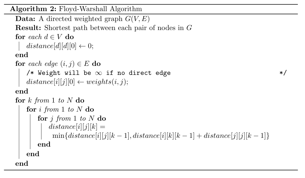
The aforementioned shortest path algorithm is not particularly efficient. In fact, we saw that uniform cost search can find the shortest path from a source node to all other nodes more efficiently, without the acyclic restriction! We will now consider the Floyd-Warshall algorithm (FW) that can compute the shortest path between all pairs of nodes in a graph in \(O(n^3)\) time! FW is a dynamic programming solution that operates on a directed graph. We assume that the edges may even have negative weights, but that there are no negative-weight cycles (otherwise the shortest path would be to loop in that cycle forever and achieve a distance of \(-\infty\)!)
Let us assume that the graph contains \(N\) nodes that are labelled \(\{1, 2, \ldots, N\}\). We define \(d_{ij}^{(k)}\) to be the length of the shortest path between \(i\) and \(j\) that only passes through nodes in the set \(\{1, 2, \ldots, k\}\). Given this, we therefore want to find the shortest path from every \(i\) to every \(j\) using any vertex in \(\{1, 2, \ldots, N\}\).
Next, denote \(p\) as the shortest path from \(i\) to \(j\) whose intermediate nodes are in the set \(\{1, 2, \ldots, k\}\). We can make the following observations:
- If the node \(k\) is not an intermediate node in the path \(p\) (i.e. \(k\) is not visited along the shortest path from \(i\) to \(j\)), then the shortest path uses only nodes in the set \(\{1, 2, \ldots, k-1\}\). We can therefore write \(d_{ij}^{(k)} = d_{ij}^{(k-1)}\)
- Otherwise, \(k\) is in the shortest path. In this case, the shortest path from \(i\) to \(j\) can be written as the shortest path from \(i\) to \(k\), plus the shortest path from \(k\) to \(j\). In other words: \(d_{ij}^{(k)} = d_{ik}^{(k-1)} + d_{kj}^{(k-1)}\)
- When \(k = 0\), we have that there should be no intermediate nodes in the path. Therefore, \(d_{ij}^{(0)} = w_{ij}\) where \(w_{ij}\) is the weight of the edge between \(i\) and \(j\) (\(\infty\) if no such edge exists).
Putting these three observations together gives us the following recursive definition:
\[ d_{ij}^{(k)} = \begin{cases} w_{ij} &\text{ if } k = 0 \\ \min \{ d_{ij}^{(k-1)}, d_{ik}^{(k-1)} + d_{kj}^{(k-1)} \} &\text{ if } k \ge 1 \\ \end{cases} \]
For any shortest path, the intermediate nodes are in the set \(\{1, 2, \ldots, N\}\). Therefore, we must simply compute the matrix of values \(d_{ij}\) for all \(i, j \in \{1, \ldots, N\}\). Each entry \((r, c)\) in this matrix indicates the cost of the shortest path between nodes \(r\) and \(c\).
We can compute this matrix bottom-up using the approach in the algorithm below.
Note that we do
After initialising the matrix of values, the algorithm executes three nested loops, each running from \(1\) to \(N\).
The work done inside the inner most loop is a constant-time operation, and so the entire algorithm runs in \(O(N^3)\)
4.4 Summary Lecture (Part 1)
The video below summarises the above sections. You may either watch it first, or read through the notes and watch it as a recap.
4.5 Making Change
Recall that the greedy approach to making change of repeatedly choosing the coin with the biggest denomination less than the change required did not always produce a solution with the minimum number of coins. Whether the greedy approach worked or not depended on the coin set being used. In this section we consider a dynamic programming solution which will always find the minimum number of coins.
Suppose that we are using a currency that has \(n\) coins of denominations \(d_i, 1 \le i \le n\) and \(0 < d_1 < d_2 < d_3 < \ldots < d_n\) . As before, we will assume that we have an infinite supply of coins of each denomination. The problem then is to give the minimum number of coins to make up some given value, say \(C\), of change.
To get an idea of how we would solve this problem let us consider making change to a value of 9 from coins of denominations 1, 2, 5. If we were to consider all three coins, we note that we could make up the solution by either using a coin of denomination 5, or we could have a solution which does not include a 5. If we do not use a 5, then our solution would be the solution to making change for 9 using only coins 1, 2. If we do use a 5, then our solution would be 1 coin plus the number of coins required to make change for 4 (i.e. \(9 − 5\)) using coins in 1, 2, 5. The required solution is whichever of these two choices results in the fewest coins.
In general, when we are trying to make change that adds up to some amount \(j\) using coins of denominations from 1 up to \(i\), then there are two choices. We might not use a coin of denomination \(i\), in which case our solution would be the number of coins required to make change for \(j\) using coins of denominations from \(1\) up to \(i − 1\). Or we might use a coin of denomination \(i\), in which case our solution would be 1 coin plus the number of coins required to make change for \(j − d_i\) using coins of denominations from \(1\) up to \(i\). Again the solution to the problem would be the one with the fewest coins.
If \(c[i, j]\) is used to denote the number of coins required to make change for \(j\) using the denomi- nations of coins from 1 up to \(i\), then we can write this choice out as
\[ c[i, j] = \min(c[i − 1, j], 1 + c[i, j − d_i]) \]
We would then build up our solution by solving the subproblems given in the equations. Again, it seems that this is inherently a recursive solution, but once again we note that if we solved the problem recursively, then we would be recalculating some results. As before, to set up a bottom-up dynamic programming solution, we will create a table to store the partial solutions from which we will make up final solution.
Here we create a table \(c[1 \ldots n, 0 \ldots C]\) with one row for each available denomination (from smallest at the top to largest at the bottom) and one column for each value of change from \(0\) to \(C\). We also set \(c[i, 0] = 0\) for all \(i\). For the example we used above, we would have the table as given below.
| Amount | 0 | 1 | 2 | 3 | 4 | 5 | 6 | 7 | 8 | 9 |
|---|---|---|---|---|---|---|---|---|---|---|
| \(d_1=1\) | 0 | |||||||||
| \(d_2=2\) | 0 | |||||||||
| \(d_3=5\) | 0 |
We then fill in the table working from top to bottom and from left to right in each row. So to fill \(c[1, 1]\) we would use the equation
\[ c[1, 1] = \min(c[1 − 1, 1], 1 + c[1, 1 − 1]) = \min(c[0, 1], 1 + c[1, 0]). \]
Note that we have to handle a special case here as \(c[0, 1]\) is undefined — we would simply use the other choice.
Then to fill \(c[1, 2]\) (making change for \(2\) using only coins from \(d_1\) ) we would use the equation
\[ c[1, 2] = \min(c[1 − 1, 2], 1 + c[1, 2 − 1]) = \min(c[0, 1], 1 + c[1, 1]) = 2, \] and so on…
Once we have filled the first row our table would be
| Amount | 0 | 1 | 2 | 3 | 4 | 5 | 6 | 7 | 8 | 9 |
|---|---|---|---|---|---|---|---|---|---|---|
| \(d_1=1\) | 0 | 1 | 2 | 3 | 4 | 5 | 6 | 7 | 8 | 9 |
| \(d_2=2\) | 0 | |||||||||
| \(d_3=5\) | 0 |
We could then start filling row 2. To fill \(c[2, 1]\) (making change for 1 using only coins from \(d_1\) and \(d_2\)) we would use the equation
\[ c[2, 1] = \min(c[2 − 1, 1], 1 + c[2, 1 − d_2 ]) = \min(c[1, 1], 1 + c[2, −1]) \]
Here \(c[2, −1]\) is undefined, so we would ignore it. \(c[1, 1] = 1\) so \(c[2, 1] = 1\) as well.
To fill \(c[2, 2]\) (making change for 2 using only coins from \(d_1\) and \(d_2\)) we would use the equation
\[ c[2, 2] = \min(c[2 − 1, 2], 1 + c[2, 2 − d_2 ]) = \min(c[1, 2], 1 + c[2, 0]) = \min(2, 1) \]
Filling in the second and third rows of the table results in
| Amount | 0 | 1 | 2 | 3 | 4 | 5 | 6 | 7 | 8 | 9 |
|---|---|---|---|---|---|---|---|---|---|---|
| \(d_1=1\) | 0 | 1 | 2 | 3 | 4 | 5 | 6 | 7 | 8 | 9 |
| \(d_2=2\) | 0 | 1 | 1 | 2 | 2 | 3 | 3 | 4 | 4 | 5 |
| \(d_3=5\) | 0 | 1 | 1 | 2 | 2 | 1 | 2 | 2 | 3 | 3 |
Here to fill \(c[3, 9]\) (making change for 9 using coins from \(d_1\), \(d_2\) and \(d_3\)) we would use the equation
\[ c[3, 9] = \min(c[3 − 1, 9], 1 + c[3, 9 − d_3 ]) = \min(c[2, 9], 1 + c[3, 9 − 5]) = \min(5, 3) \]
Note that in general if either \(i = 1\) or \(j < d_i\), then one of the terms used in finding the minimum in the equation is undefined and we would just use the other term. If \(i = 1\) and \(j < d_i\), then we have a situation where it is impossible to pay an amount of \(j\) using coins from \(d_1\) only. In this case we would set \(c[i, j] = \infty\).
The algorithm for this dynamic programming solution is given in Algorithm 2.
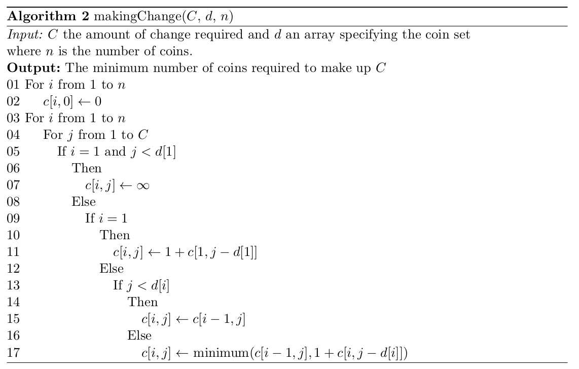
We now need to consider the efficiency of our algorithm. Here all that we need to do to find the minimum number of coins required to give change for \(C\) is to fill the array \(c\). First we set \(c[i, 0]\) to be \(0\) for all \(i\) and then we fill \(n \times C\) other positions in the array. Filling each position in the array takes constant time so the algorithm is \(O(nC)\) overall.
Proving that our solution method is correct can be done in a similar fashion to the proof that the shortest path solution is correct and follows directly from the observation that
\[ c[i, j] = \min(c[i − 1, j], 1 + c[i, j − d_i ]), \forall i = 1, \ldots, n \text{ and } j = 0, \ldots , C \]
4.6 Efficient Matrix Multiplication
Suppose we have to tackle the problem of finding the product of a number of matrices while doing the least amount of work to multiply them together. Recall that to multiply a \(m \times n\) matrix and a \(n \times p\) matrix together we do \(m \times n \times p\) multiplications. As an example of our problem, consider multiplying together the three matrices \(M_1\) , \(M_2\) and \(M_3\) where \(M_1\) is \(3 \times 4\), \(M_2\) is \(4 \times 2\) and \(M_3\) is \(2 \times 8\). There are two distinct orders in which to do the multiplication (as shown by the parenthesisation below).
- \((M_1M_2)M_3\) which involves \(3 \times 4 \times 2 + 3 \times 2 \times 8 = 24 + 48 = 72\) multiplications, and
- \(M_1 (M_2 M_3)\) which involves \(4 \times 2 \times 8 + 3 \times 4 \times 8 = 64 + 96 = 160\) multiplications.
A considerable difference in the amount of work done!
In the remainder of this section we consider a dynamic programming solution to the problem below (see Chapter 15 of Introduction to Algorithms) for a detailed discussion) .
Problem: Given a chain of 2-dimensional matrices \(M_1 , M_2 , \ldots , M_n\) (where \(M_i\) has dimensions \(d_{i−1} \times d_i\) for all \(1 \le i \le n\)) to be multiplied together, determine the order in which the muliplications must be made in order to do the least amount of work.
Once again we see that one way to solve this problem would be a recursive solution. Let us begin by defining \(m(i, j)\) to be the minimum number of multiplications to compute \(M_i \times \ldots \times M_j , 1 \le i < j \le n\). Here \(m(1, n)\) would be the solution we are looking for — the minimum number of multiplications to calculate \(M_1 \times M_2 \times \ldots \times M_n\). Note that to calculate \(m(i, j)\) for any \(i\) and \(j\), we would have to consider all of the possible parenthesisations of this subproblem. We could however split this subproblem up further by recognising that the best way to multiply these matrices together would be splitting this chain at every possible position and picking the minimum of these results. That is
\[ m(i, j) = \min\limits_{i \le k < j} (m(i, k) + m(k + 1, j) + d_{i−1} d_k d_j), 1 \le i < j \le n. \]
Note that \(m(h, h) = 0\) for \(1 \le h \le n\).
Once again we would not actually want to solve this problem in a recursive fashion as it would mean that some subproblems are solved repeatedly. Instead we use the ideas of dynamic programming and build up the solution of our problem bottom-up. To do this we create a table of solutions to subproblems. This table is actually an upper triangular matrix which we will fill from the main diagonal where all the entries are 0 and work towards the top right corner which is where our final solution will be found.
To see how this works consider the problem of multiplying 5 matrices together. Note that all the information that is required are the dimensions of the matrices, so let
| Dimension | Value |
|---|---|
| \(d_0\) | 3 |
| \(d_1\) | 2 |
| \(d_2\) | 3 |
| \(d_3\) | 4 |
| \(d_4\) | 5 |
| \(d_5\) | 2 |
Then to build up \(m\) we first set all elements on the main diagonal to be 0 as shown below.
| 1 | 2 | 3 | 4 | 5 | |
|---|---|---|---|---|---|
| 1 | 0 | ||||
| 2 | - | 0 | |||
| 3 | - | - | 0 | ||
| 4 | - | - | - | 0 | |
| 5 | - | - | - | - | 0 |
Then we calculate all the values one off the main diagonal, i.e. \(m(1, 2), m(2, 3)\) etc. as shown below. Here \(m(1, 2) = d_0d_1 d_ 2\) , \(m(2, 3) = d_1 d_2 d_3\) etc.
| 1 | 2 | 3 | 4 | 5 | |
|---|---|---|---|---|---|
| 1 | 0 | 18 | |||
| 2 | - | 0 | 24 | ||
| 3 | - | - | 0 | 60 | |
| 4 | - | - | - | 0 | 40 |
| 5 | - | - | - | - | 0 |
Then we calculate the next set of values — \(m(1, 3), m(2, 4), m(3, 5)\) by considering \(m(1, 2)\) and \(m(2, 3)\) for \(m(1, 3)\), etc. Here
\[ m(1, 3) = \min(m(1, 1) + m(2, 3) + d_0 d_1 d_3 , m(1, 2) + m(3, 3) + d_0 d_2 d_3) \] \[ m(1, 3) = \min(0 + 24 + 24, 18 + 0 + 36) = \min(48, 54) = 48, \] etc.
| 1 | 2 | 3 | 4 | 5 | |
|---|---|---|---|---|---|
| 1 | 0 | 18 | 48 | ||
| 2 | - | 0 | 24 | 64 | |
| 3 | - | - | 0 | 60 | 64 |
| 4 | - | - | - | 0 | 40 |
| 5 | - | - | - | - | 0 |
Then we do the same for the next diagonal, \(m(1, 4)\) and \(m(2, 5)\)
| 1 | 2 | 3 | 4 | 5 | |
|---|---|---|---|---|---|
| 1 | 0 | 18 | 48 | 94 | |
| 2 | - | 0 | 24 | 64 | 76 |
| 3 | - | - | 0 | 60 | 64 |
| 4 | - | - | - | 0 | 40 |
| 5 | - | - | - | - | 0 |
And so on until we get
| 1 | 2 | 3 | 4 | 5 | |
|---|---|---|---|---|---|
| 1 | 0 | 18 | 48 | 94 | 88 |
| 2 | - | 0 | 24 | 64 | 76 |
| 3 | - | - | 0 | 60 | 64 |
| 4 | - | - | - | 0 | 40 |
| 5 | - | - | - | - | 0 |
\(m(1, n)\) then contains the minimum number of multiplications to multiply the matrices together.
The algorithm to find the minimum number of multiplications required to multiply the matrices together is given in Algorithm 3.
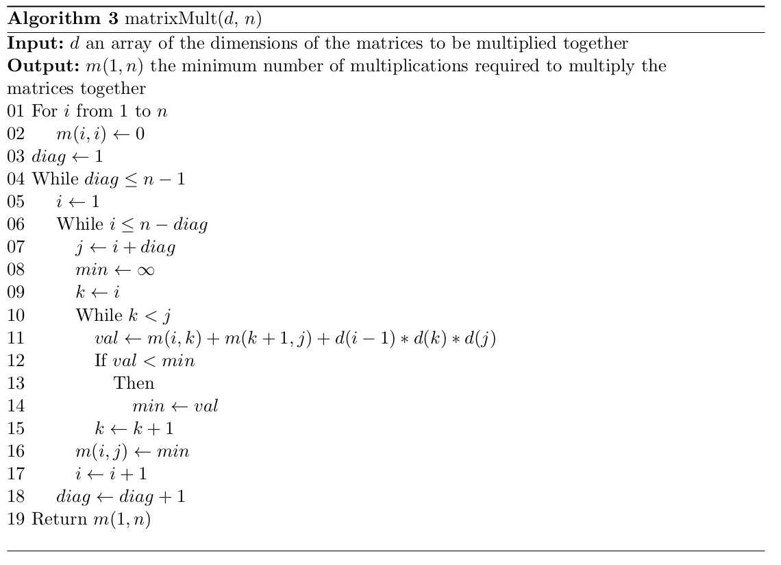
Let us now consider the efficiency of the algorithm. The algorithm calculates values for around half the positions in the matrix \(m\). That is, around \(\dfrac{n^2}{2}\) matrix entries. The work done for each entry involves finding the best value for that particular entry in the matrix by testing all possible positions of \(k\) between \(i\) and \(j\). There are at most \(n\) of these positions. For each position of \(k\), two matrix lookups, two multiplications and three additions are done. That is, a small number of constant time operations. Finding the best split is thus \(O(n)\) and so the algorithm is \(O(n^3)\) overall. Note that the algorithm does, however, require \(O(n^2)\) space.
To prove that the algorithm is correct we would once again use an inductive approach based on the fact that for each subproblem we test all the possible solutions to find the minimum and we build up our final solution from the optimal solutions to various subproblems.
Note that the algorithm above does not actually return the optimal factorisation (it only gives the minimum number of multiplications in the optimal factorisation), but that a simple extension to the algorithm (see https://en.wikipedia.org/wiki/Matrix_chain_multiplication) can be made to get this information.
4.7 Additional Reading
- Introduction to Algorithms (Chapter 15), Cormen, Leisersin, Rivest and Stein, 3rd ed.
- https://www.geeksforgeeks.org/dynamic-programming/
- https://www.geeksforgeeks.org/floyd-warshall-algorithm-dp-16/