Chapter 9 Balanced Trees

9.1 Why Balance Matters

Every operation on a binary search tree – contains, insert, remove, min, max – traverses a single path down from the root. The work done is proportional to the length of that path, so each of these operations takes \(O(h)\) time, where \(h\) is the height of the tree.

If the tree is close to complete, with every level full except possibly the last, \(h\) is roughly \(\log n\) and everything is fast. But nothing in the BST rules keeps the tree that tightly packed. The shape depends entirely on the order in which keys are inserted, and one of the worst orders is easy to hit: keys that arrive already sorted, or nearly sorted, such as increasing IDs or timestamps.

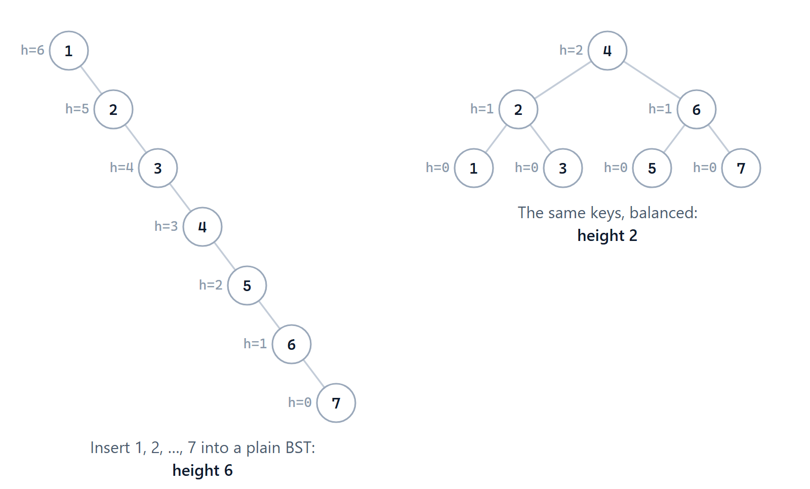
Figure 9.1: The same seven keys in two BSTs. Inserting them in sorted order gives a tree that is really just a linked list.

With a million keys, the difference is dramatic: a balanced tree has height around 19, so a search takes at most 20 comparisons. The degenerate tree has height 999,999, so a search can take a million comparisons – no better than scanning an unsorted array.

A balanced search tree adds one extra rule to the BST that forces the height to stay \(O(\log n)\), and repairs that rule after every insertion and deletion. There are many kinds of balanced tree – red-black trees (which std::map and std::set use), B-trees (used by databases and file systems), splay trees and more. In this chapter we study the first and simplest of these: the AVL tree, published by Adelson-Velskii and Landis in 1962.

9.2 AVL Trees

An AVL tree is a binary search tree plus a balance condition. To state the condition, we first need to be precise about heights.

9.2.1 Height and Balance

The height of a node is the number of edges on the longest path from that node down to a leaf. We define it recursively:

\[h(\texttt{NULL}) = -1, \qquad h(x) = 1 + \max\big(h(x.\text{left}),\ h(x.\text{right})\big).\]

So a leaf has height \(1 + \max(-1, -1) = 0\), a node whose tallest child is a leaf has height 1, and so on. Defining the empty tree to have height \(-1\) makes this formula work everywhere, with no special cases.

The balance factor of a node compares the heights of its two subtrees:

\[\text{bf}(x) = h(x.\text{left}) - h(x.\text{right}).\]

A node with a positive balance factor is left-heavy, one with a negative balance factor is right-heavy, and one with balance factor 0 is balanced. A node with balance factor \(+2\) is doubly left-heavy, and one with \(-2\) is doubly right-heavy.

The AVL condition. For every node \(x\) in the tree,

\[|\text{bf}(x)| = \big|h(x.\text{left}) - h(x.\text{right})\big| \le 1,\]

i.e. every balance factor is \(-1\), \(0\) or \(+1\). An AVL tree is a BST in which every node satisfies this condition.

In the figures and widgets in this chapter, each node’s height is written to its left, and a mark above each node shows its balance, as we draw it in lectures: a flat bar (—) when the node is balanced (0), a single arrow pointing to the heavy side when it is left-heavy (←, +1) or right-heavy (→, −1), and a red arrow with a double shaft (⇐ or ⇒) when it is doubly left-heavy (+2) or doubly right-heavy (−2), which breaks the AVL condition.

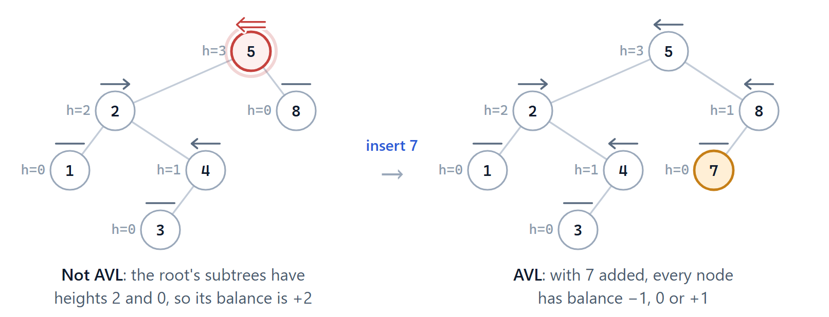
Figure 9.2: Inserting 5, 2, 1, 4, 3, 8 gives a tree that is not AVL: the root has balance +2. Adding 7 raises the height of 8, and every node is then within ±1.

The condition has to hold at every node, not just the root. A tree can look perfectly reasonable from the top and still be broken further down:

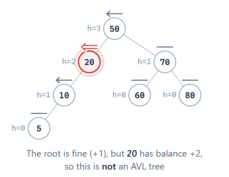
Figure 9.3: The root has balance +1, but node 20 has a left subtree of height 1 and an empty right subtree (height -1), so its balance is +2.

9.2.2 How Tall Can an AVL Tree Be?

The AVL condition doesn’t force the tree to be perfectly balanced – subtrees are allowed to differ in height by one. So how tall can an AVL tree with \(n\) nodes get? To answer this, flip the question around: what is the fewest nodes an AVL tree of height \(h\) can have? Call this number \(S(h)\).

To build the sparsest possible AVL tree of height \(h\), take a root, give it one subtree of height \(h-1\) (it needs one to have height \(h\)), and make the other subtree as short as the AVL condition allows: height \(h-2\). Both subtrees should themselves be as sparse as possible, which gives the recurrence

\[S(h) = S(h-1) + S(h-2) + 1, \qquad S(0) = 1,\quad S(1) = 2.\]

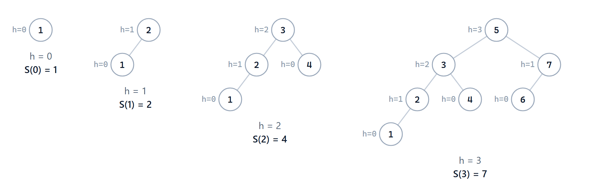
Figure 9.4: The sparsest AVL trees of heights 0 to 3. Each is a root with the two previous trees as its subtrees.

\(h\)	0	1	2	3	4	5	6	7	8	9	10
\(S(h)\)	1	2	4	7	12	20	33	54	88	143	232

This looks a lot like the Fibonacci sequence, and it is. If we let \(u(h) = S(h) + 1\), then

\[u(h) = S(h-1) + S(h-2) + 2 = u(h-1) + u(h-2),\]

which is exactly the Fibonacci recurrence, with \(u(0) = 2\) and \(u(1) = 3\). Using the usual Fibonacci numbering (\(F_0 = 0\), \(F_1 = 1\), \(F_2 = 1\), \(F_3 = 2\), \(F_4 = 3\), …), that means \(u(h) = F_{h+3}\), so

\[S(h) = F_{h+3} - 1.\]

The Fibonacci numbers grow exponentially – \(F_i \approx \varphi^i / \sqrt{5}\), where \(\varphi = \frac{1+\sqrt5}{2} \approx 1.618\) is the golden ratio. An AVL tree of height \(h\) therefore has at least roughly \(\varphi^{h+3}/\sqrt5\) nodes. Turning that around – given \(n\) nodes, how large can \(h\) be? – and taking logarithms gives the classic bound (Weiss 2014):

\[h \;\le\; 1.44 \log_2(n+2) - 1.328.\]

(The 1.44 is \(1/\log_2\varphi\): converting a base-\(\varphi\) logarithm into a base-2 logarithm.)

The height of an AVL tree is \(O(\log n)\). In fact it is at most about 44% taller than a perfectly balanced tree. Since every search follows one path from the root, a search in an AVL tree takes \(O(\log n)\) time in the worst case – not just on average.

Optional: proving the closed form for \(F_i\). The approximation above comes from Binet’s formula,

\[F_i = \frac{1}{\sqrt5}\left(\frac{1+\sqrt5}{2}\right)^i - \frac{1}{\sqrt5}\left(\frac{1-\sqrt5}{2}\right)^i = \frac{\varphi^i - \psi^i}{\sqrt5},\]

where \(\psi = \frac{1-\sqrt5}{2} \approx -0.618\). Since \(|\psi| < 1\), the \(\psi^i\) term shrinks to 0, which is why \(F_i \approx \varphi^i/\sqrt5\). We can prove the formula by strong induction on \(i\).

Base cases. For \(i = 0\): \(\frac{1}{\sqrt5}(1 - 1) = 0 = F_0\). For \(i = 1\): \(\frac{1}{\sqrt5}\left(\frac{1+\sqrt5}{2} - \frac{1-\sqrt5}{2}\right) = \frac{1}{\sqrt5}\cdot\sqrt5 = 1 = F_1\).

Inductive step. Assume the formula holds for \(F_{i-1}\) and \(F_{i-2}\). Both \(\varphi\) and \(\psi\) are roots of \(x^2 = x + 1\) (check: \(\varphi^2 = \frac{6 + 2\sqrt5}{4} = \frac{3+\sqrt5}{2} = \varphi + 1\), and similarly for \(\psi\)). So

\[F_{i-1} + F_{i-2} = \frac{\varphi^{i-2}(\varphi + 1) - \psi^{i-2}(\psi + 1)}{\sqrt5} = \frac{\varphi^{i-2}\varphi^2 - \psi^{i-2}\psi^2}{\sqrt5} = \frac{\varphi^i - \psi^i}{\sqrt5},\]

which is the formula for \(F_i\). By the principle of mathematical induction, it holds for all \(i \ge 0\). \(\blacksquare\)

9.3 Keeping the Tree Balanced

Insertion and deletion must preserve the AVL property. If we insert into an AVL tree exactly as we would into a normal BST, the new leaf can make some subtree too tall:

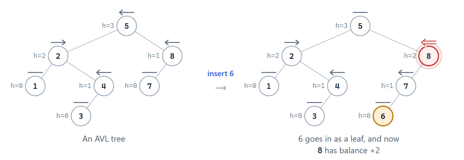
Figure 9.5: Inserting 6 as a normal BST leaf makes 8’s left subtree height 1 while its right subtree is still empty (height -1): balance +2.

Notice which nodes can be affected. Adding or removing a node only changes the heights of the nodes on the path from that node back up to the root – nothing else in the tree has changed, so nothing else can have become unbalanced.

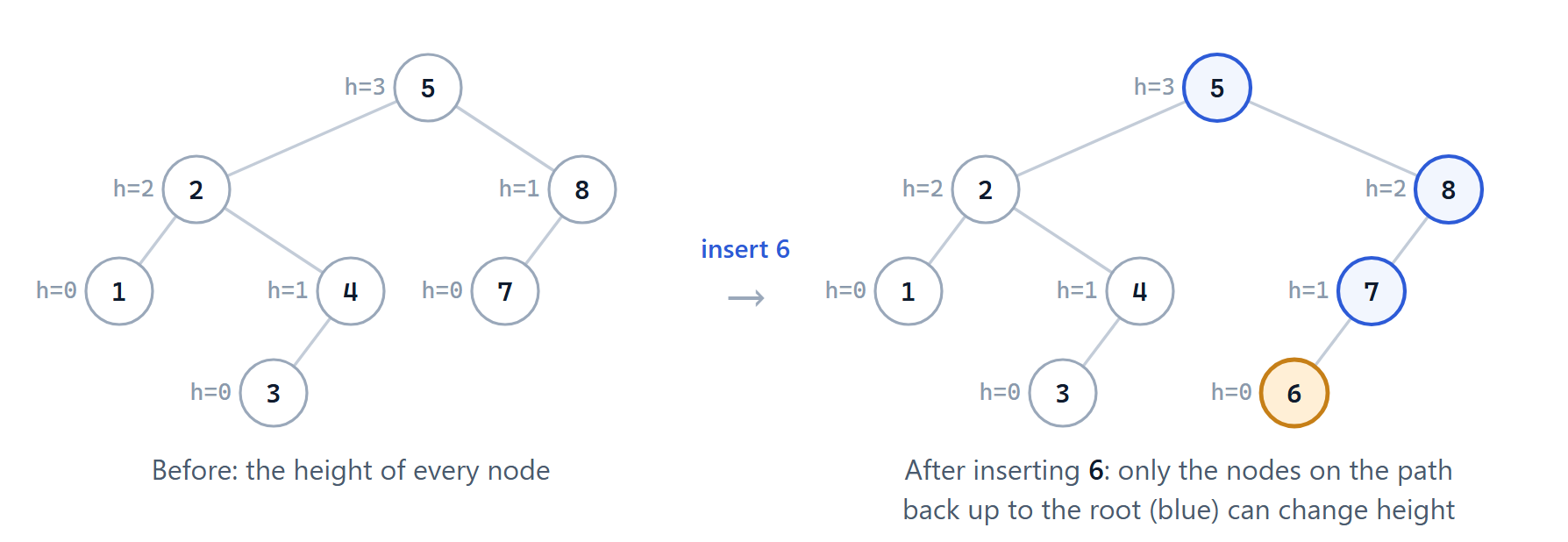
Figure 9.6: Inserting 6 can only change the heights of the nodes on the path from 6 back up to the root: 7, 8 and 5. Here 7 and 8 each grow by one, while 5 stays at height 3 because its left subtree was already that tall. Every other node keeps its height, so it keeps its balance too.

So after an insertion or deletion, we traverse back up that path updating heights, and at the lowest node that has become unbalanced (call it the problem node) we repair the tree. The repair tool is called a rotation.

9.3.1 Rotations

A rotation is a small, local rearrangement of three pointers that moves one node up and its parent down, without violating the search property: every key in a node’s left subtree is still smaller than it, and every key in its right subtree is still larger, so the tree is still a valid BST afterwards.

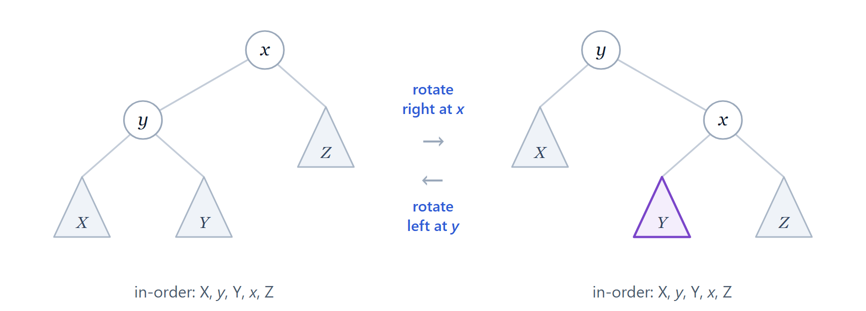
Figure 9.7: Rotating right at x makes its left child y the root of this subtree, with x as y’s right child. The only subtree that changes parent is Y. Rotating left at y undoes it. Reading left to right, the order X, y, Y, x, Z is the same in both.

To rotate right at \(x\): \(x\)’s left child \(y\) moves up into \(x\)’s place, \(x\) becomes \(y\)’s right child, and \(y\)’s old right subtree (\(Y\)) becomes \(x\)’s new left subtree. It has to go somewhere, and it fits there perfectly: every key in \(Y\) is bigger than \(y\) but smaller than \(x\). Rotate left is the mirror image. Either way, only a constant number of pointers change, so a rotation takes \(O(1)\) time.

Notation. We write RR(\(x\)) for rotate right at \(x\) and LR(\(x\)) for rotate left at \(x\). A double rotation is then just two of these in a row, for example LR(6) followed by RR(8). Be careful: many textbooks and websites use the letters LL, LR, RL and RR for the four cases instead, which is easy to mix up. In this book RR and LR always name a rotation, and the cases are always named in words: “the left-left case”, “the left-right case”, and so on.

The widget below shows exactly what rotations do to the heights, using triangles for whole subtrees whose contents don’t matter. Step through the single rotation first, then see why it doesn’t work when the extra height is on the inside, and how a double rotation fixes that. Whenever a rotation is needed, you do it: grab the node that should move up and drag it onto its parent. As you drag, the tree morphs into its rotated shape; let go past halfway to commit the rotation (or press Show me if you’re stuck). The side buttons switch to the mirror-image (right-heavy) versions.

Open in new tab ↗

9.3.2 The Four Cases

Suppose \(p\) is the problem node, so its balance is \(+2\) or \(-2\). Which rotations fix it depends on two things: which side \(p\) is heavy on, and which side that child is heavy on. Label the heavy child \(c\):

p is…	its heavy child c is…	Case	Fix
doubly left-heavy, +2	left-heavy, +1	left-left	RR(p)
doubly left-heavy, +2	right-heavy, −1	left-right	LR(c), then RR(p)
doubly right-heavy, −2	right-heavy, −1	right-right	LR(p)
doubly right-heavy, −2	left-heavy, +1	right-left	RR(c), then LR(p)

Left-left and right-right are mirror images of each other. The extra height is on the outside of the tree (the left child of a left child, or the right child of a right child), and a single rotation fixes it. Left-right and right-left are also mirror images, but the extra height is on the inside, and they need a double rotation.

9.3.3 Single Rotations: the Outside Cases

In the left-left case, the problem node \(x\) has a left child \(y\) that is also left-heavy: the new node went into \(y\)’s left subtree. Rotating right at \(x\) lifts that tall subtree up by one level and drops \(x\)’s short side down by one, and everything evens out.

There is a second, very important thing to notice about this. Before the insertion, the subtree rooted at \(x\) had height \(h+1\). The insertion made it \(h+2\) – but after the rotation, the subtree (now rooted at \(y\)) has height \(h+1\) again. As far as the rest of the tree is concerned, nothing changed. So no node further up can be unbalanced any more, and one rotation is always enough to fix an insertion.

Example. Insert 6 into the tree from before. 6 goes in as the left child of 7. Traversing back up, 7 is fine (+1), but 8 has balance \(+2\). Its left child 7 is left-heavy, so this is a left-left case: rotate right at 8, RR(8).

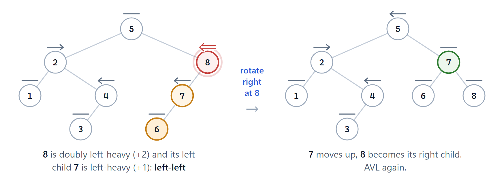
Figure 9.8: Left-left: rotate right at 8.

Example. Insert 5 into the tree \(6, 2, 8, 4, 7\). It goes to the right of 4. Traversing back up, 4 is fine (\(-1\)) but 2 has balance \(-2\), and its right child 4 is right-heavy: a right-right case. Rotate left at 2, LR(2).

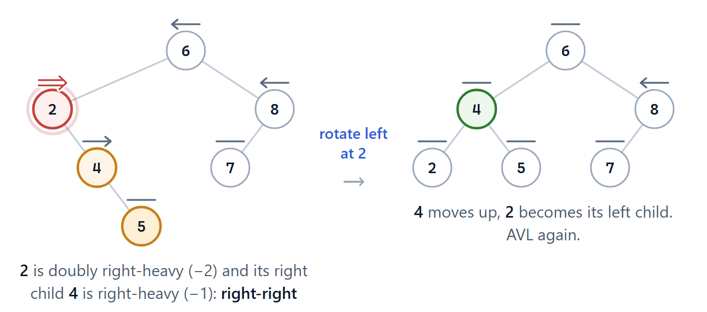
Figure 9.9: Right-right: rotate left at 2.

9.3.4 Double Rotations: the Inside Cases

Now insert 7 into the tree \(5, 2, 8, 1, 4, 6, 3\). It goes to the right of 6. Node 8 has balance \(+2\) again, so it’s doubly left-heavy – but this time its left child 6 is right-heavy. What happens if we try the same single rotation?

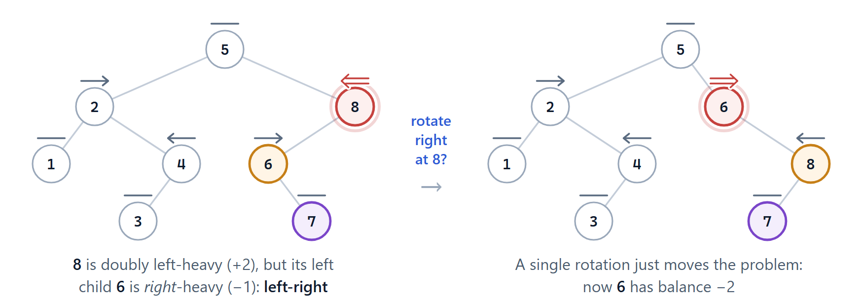
Figure 9.10: A single rotation doesn’t fix an inside case: the tall middle subtree just moves across to the other side, and the problem is mirrored rather than solved.

The extra height is in the middle of the subtree – in the right subtree of the left child – and a rotation only moves the middle subtree from one side to the other. The fix is to do two rotations:

1. Rotate at the child \(c\), in the direction that turns the inside case into an outside case. Here, rotating left at 6 lifts 7 up, and now 8’s left child is left-heavy: a left-left case.
2. Rotate at the problem node \(p\) in the other direction, exactly as for the outside case. Here, rotate right at 8.

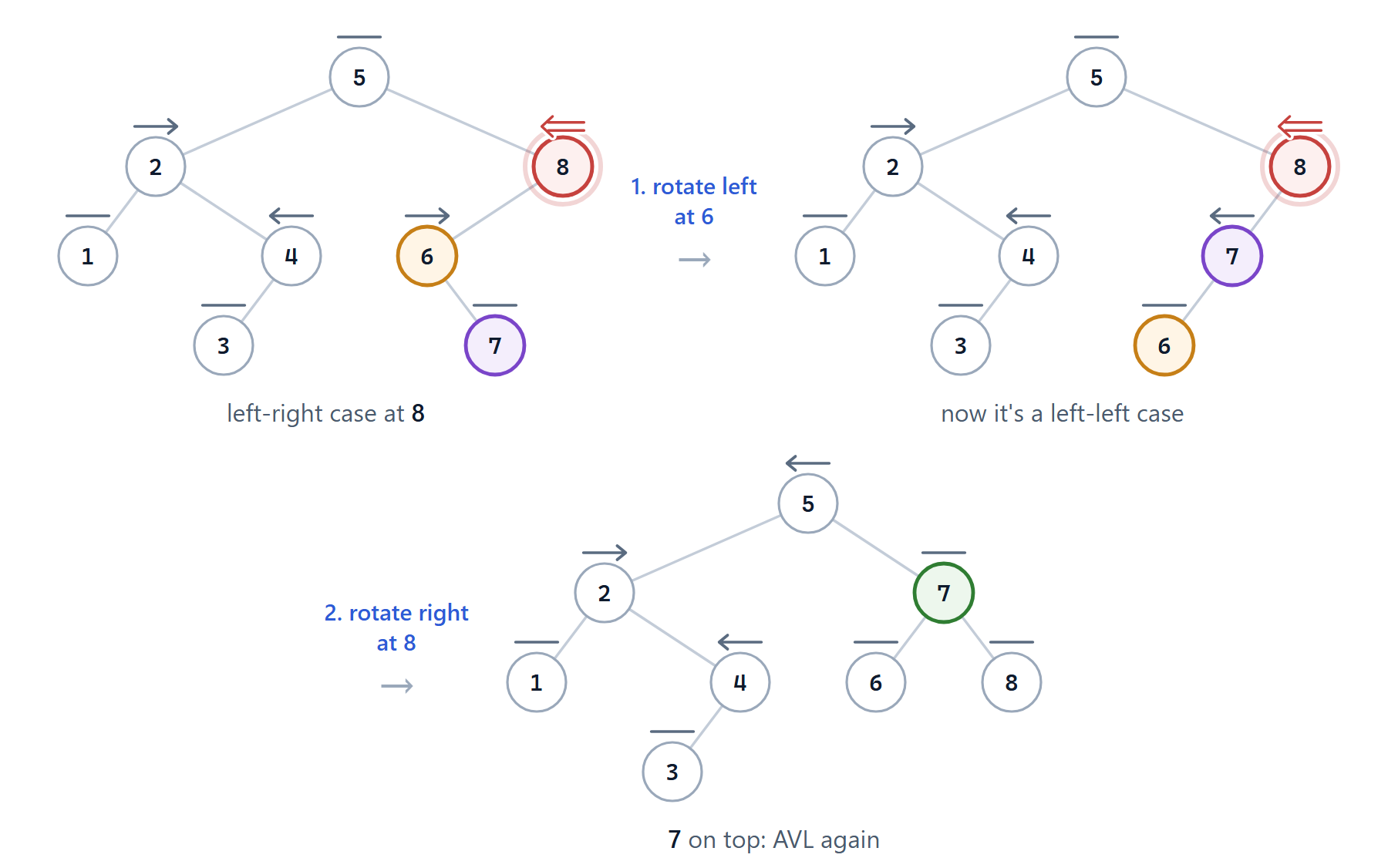
Figure 9.11: Left-right: rotate left at 6, then rotate right at 8.

Rule of thumb for the inside cases. The problem node \(p\), its child \(c\) and its grandchild \(g\) (the one the new key was inserted under) are rearranged so that the grandchild ends up on top, with \(c\) and \(p\) as its two children. Just like the single rotation, this restores the subtree’s original height, so one double rotation is enough to fix any insertion.

9.3.5 Putting It Together

The whole rebalancing step:

Pseudocode: rebalancing the problem node \(p\).

if p is doubly left-heavy (bf(p) = +2):
    if p.left is left-heavy or balanced:      // left-left
        rotate right at p
    else:                                     // left-right
        rotate left at p.left
        rotate right at p

else if p is doubly right-heavy (bf(p) = -2):
    if p.right is right-heavy or balanced:    // right-right
        rotate left at p
    else:                                     // right-left
        rotate right at p.right
        rotate left at p

(The “or balanced” only matters for deletion – after an insertion, the heavy child is never perfectly balanced. We’ll see why when we get to deletion.)

So inserting into an AVL tree is:

1. Insert the key as a new leaf, exactly as in a normal BST.
2. Traverse back up the path towards the root, updating each node’s height.
3. At the first node that’s unbalanced, apply the fix above. Stop: the subtree’s height is back to what it was, so the rest of the tree is fine.

In C++

Recomputing heights recursively every time we need a balance factor would take \(O(n)\) time, which would defeat the whole point. Instead, each node stores its height, and we update it whenever the node’s children change.

class TreeNode {
public:
    TreeNode *left = nullptr;
    TreeNode *right = nullptr;
    int value;
    int height = 0;                 // a new leaf has height 0

    TreeNode(int v) : value(v) {}
};

int height(TreeNode *n) { return n == nullptr ? -1 : n->height; }
int balance(TreeNode *n) { return height(n->left) - height(n->right); }
void updateHeight(TreeNode *n) {
    n->height = 1 + std::max(height(n->left), height(n->right));
}

A rotation takes the subtree’s root pointer by reference – exactly like insert(int v, TreeNode *&subtree) in the BST lab – so it can swing whichever pointer used to point at \(x\) (the root, or the parent’s left or right) over to the new subtree root. For RR(\(x\)): \(x\)’s left child \(y\) moves up, \(y\)’s old right subtree becomes \(x\)’s new left subtree, \(x\) becomes \(y\)’s right child, and the pointer that used to point at \(x\) now points at \(y\). LR(\(x\)) is the mirror image. Writing these two functions is part of the lab.

Because the recursive insert naturally traverses back up the path as each call returns, rebalancing slots in right after the recursive call. The whole of AVL insertion is then one function:

Pseudocode: AVL insert.

insert(v, subtree):
    // 1. insert exactly as in a normal BST
    if subtree is empty:
        subtree = new node(v)                      // a new leaf has height 0
        return
    if v < subtree.value:
        insert(v, subtree.left)
    else:
        insert(v, subtree.right)

    // 2. on the way back up: update this node's height
    subtree.height = 1 + max(height(subtree.left), height(subtree.right))

    // 3. check the balance and fix whichever case it is
    if balance(subtree) = +2:                      // doubly left-heavy
        if balance(subtree.left) >= 0:             // left-left
            RR(subtree)
        else:                                      // left-right
            LR(subtree.left)
            RR(subtree)
    else if balance(subtree) = -2:                 // doubly right-heavy
        if balance(subtree.right) <= 0:            // right-right
            LR(subtree)
        else:                                      // right-left
            RR(subtree.right)
            LR(subtree)

Here height(empty) is \(-1\) and balance(n) is height(n.left) - height(n.right).

Update heights bottom-up. After a rotation, the node that moved down must have its height updated before the node that moved up, because the new parent’s height depends on its children’s. Getting this order wrong is the most common AVL bug – and it’s silent: the tree still looks like a valid BST, but its stored heights are wrong, so later rotations happen in the wrong places.

The playground below runs the whole algorithm, one narrated step at a time. Load the worked examples from this chapter, or type in your own keys. Try inserting 1 to 7 in order with AVL balancing on, then again with it switched off. You can also rotate by hand at any time by dragging a node up onto its parent. With balancing off, try building a degenerate tree and then balancing it yourself with rotations.

Open in new tab ↗

9.4 Deletion

Deletion works the same way: delete the node exactly as in a normal BST (a leaf is removed, a node with one child is replaced by that child, and a node with two children is replaced by its in-order successor), then traverse back up from where a node was physically removed, updating heights and rebalancing. Often nothing needs fixing at all:

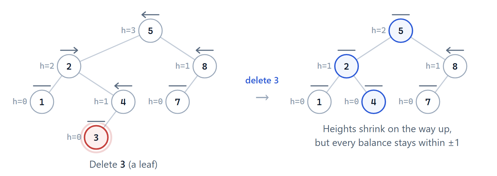
Figure 9.12: Deleting 3 shrinks the heights of 4, 2 and 5, but no balance factor goes outside ±1, so no rotation is needed.

When something does go wrong, the same four cases and the same rotations fix it. Deleting a node makes one side of an ancestor shorter, which is the same as making the other side taller – so the problem node is heavy on the side opposite to the deletion.

Example. Delete 32 from the tree below. Node 44’s left subtree drops to height 0 while its right subtree still has height 2: balance \(-2\). It’s doubly right-heavy, and its right child 78 is left-heavy (\(+1\)), so this is a right-left case. Rotate right at 78, then left at 44: RR(78) followed by LR(44).

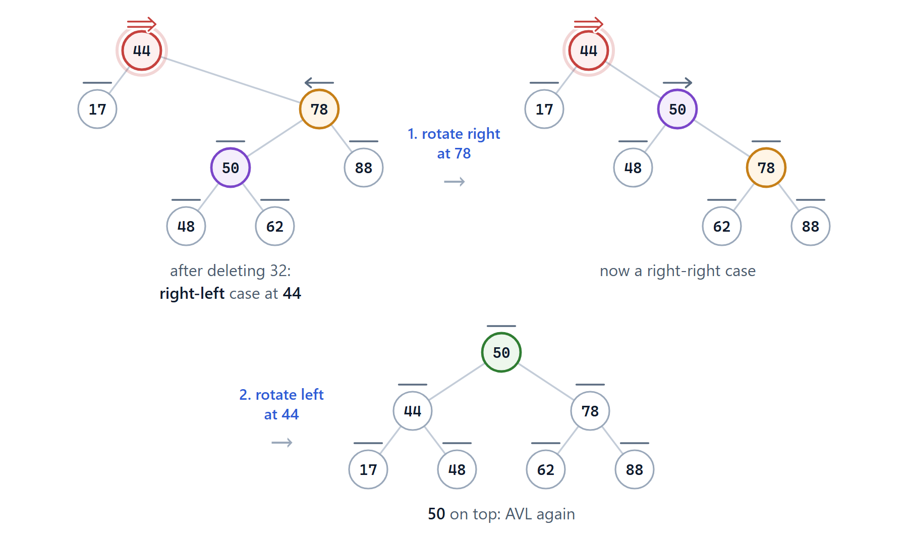
Figure 9.13: Deleting 32 leaves a right-left case at 44: rotate right at 78, then rotate left at 44.

There are two differences from insertion to watch out for:

1. The heavy child can be balanced. After a deletion, the problem node’s heavy child can have balance factor 0 – both of its subtrees equally tall. (This can’t happen after an insertion.) In that case, use a single rotation, as for an outside case. That’s what the “or balanced” in the pseudocode is for. A double rotation here can leave the tree unbalanced.
2. One fix might not be enough. After an insertion, a rotation restores the subtree’s old height, so the rest of the tree can’t tell anything happened. After a deletion, the subtree was already one level shorter than it used to be, and a rotation can shrink it by one more – which can unbalance a node further up. So we must keep traversing all the way back up to the root, and there might be a rotation needed at every level. That is still only \(O(\log n)\) rotations, each taking \(O(1)\) time.

Deletion therefore looks just like insertion: do the normal recursive BST removal, and then, on each node as the recursion returns, update its height and check its balance exactly as in steps 2 and 3 of the insert pseudocode. Since that runs at every level on the way back up, the cascading case is handled automatically.

9.5 Complexity

Operation	BST (worst case)	AVL tree (worst case)	Notes
contains	\(O(n)\)	\(O(\log n)\)	one root-to-leaf path
min / max	\(O(n)\)	\(O(\log n)\)	follow left / right pointers
insert	\(O(n)\)	\(O(\log n)\)	at most one single or double rotation
remove	\(O(n)\)	\(O(\log n)\)	possibly one rotation per level: \(O(\log n)\) total
In-order traversal	\(O(n)\)	\(O(n)\)	every node is visited once
Rotation	–	\(O(1)\)	a few pointer changes and two height updates

The price for all of this is small: one extra int per node to store its height, and a little extra work on the way back up after each insertion or deletion.

AVL trees vs. red-black trees. The balanced trees in the C++ standard library (std::map, std::set) are usually red-black trees. Their rule is looser – the height can be up to \(2\log_2(n+1)\), rather than about \(1.44\log_2 n\) – so they need fewer rotations when the tree changes, while AVL trees are a little more tightly balanced, which makes lookups slightly faster. Both guarantee \(O(\log n)\) for every operation.

9.6 Practice

Two kinds of exercise, in the same format as the BST practice widget. Spot the imbalance: decide which nodes (if any) break the AVL condition, working out the heights yourself. Fix the tree: after an insertion or deletion, find the problem node, name the case, and then do the rotations yourself by dragging nodes up onto their parents. The case buttons let you drill a particular case, and Show steps through the answer.

Open in new tab ↗

9.7 Lab: AVL Trees

For this lab, you will turn a binary search tree into an AVL tree. Like the BST lab, it is graded using unit tests: you submit a single implementation file, and the tests call the methods of your AVLTree class directly.

Most of the class is given to you. You need to implement three things:

1. rotateRight
2. rotateLeft
3. the rebalancing part of insert

9.7.1 The Header

Implement your AVL tree against the following header – do not change it:

#ifndef AVL_H
#define AVL_H

class TreeNode
{
public:
    TreeNode *left = nullptr;
    TreeNode *right = nullptr;
    int value;
    int height = 0;                 // a new leaf has height 0

    TreeNode(int v) : value(v) {}
};

class AVLTree
{
public:
    TreeNode *root = nullptr;

    void insert(int value);
    bool contains(int value);
    void preOrderTraversal();
    void inOrderTraversal();

    // Rotations are public so that the unit tests can call them directly
    void rotateRight(TreeNode *&x);
    void rotateLeft(TreeNode *&x);

    ~AVLTree();

private:
    int height(TreeNode *n) const;  // -1 for an empty subtree
    int balance(TreeNode *n) const; // height(left) - height(right)
    void updateHeight(TreeNode *n); // 1 + the larger child height

    void insert(int v, TreeNode *&subtree);
    bool contains(int value, TreeNode *subtree) const;
    void preOrderTraversal(TreeNode *subtree) const;
    void inOrderTraversal(TreeNode *subtree) const;
};

#endif // AVL_H

Given: the public insert and contains, both traversals (which print each value followed by a space, as in the BST lab), the destructor, and the three helpers height, balance and updateHeight:

int AVLTree::height(TreeNode *n) const { return n == nullptr ? -1 : n->height; }
int AVLTree::balance(TreeNode *n) const { return height(n->left) - height(n->right); }
void AVLTree::updateHeight(TreeNode *n) {
    n->height = 1 + std::max(height(n->left), height(n->right));
}

9.7.2 Rotations

Implement rotateRight and rotateLeft, using the description in Putting It Together and Figure 9.7. Each one takes the root of a subtree by reference, rearranges the pointers, and leaves x pointing at the new root of the subtree. Don’t forget to update the heights of the two nodes that moved – the one that moved down first.

For example, take the tree with root 8, whose left child is 7, whose left child is 6 (built by hand, so it isn’t balanced). After rotateRight(root), root should point at 7, with 6 and 8 as its children, and the stored heights should be 1 for 7 and 0 for 6 and 8. rotateLeft is the mirror image: on the tree 2 → 4 → 5 (each node the right child of the one before), rotateLeft(root) should leave 4 at the root with children 2 and 5.

The unit tests call your rotations on trees like these directly, so they must work on any subtree, not just as part of insert.

9.7.3 Insert

The given code contains steps 1 and 2 of the insert pseudocode – the normal BST insertion and the height update. Complete step 3: check the balance of subtree and apply the right rotations for each of the four cases.

void AVLTree::insert(int v, TreeNode *&subtree) {
    if (subtree == nullptr) {
        subtree = new TreeNode(v);
        return;
    }
    if (v < subtree->value) insert(v, subtree->left);
    else                    insert(v, subtree->right);

    updateHeight(subtree);

    // TODO: if subtree is doubly left-heavy or doubly right-heavy,
    //       work out which of the four cases it is and rotate.
}

To test it, insert 1, 2, 3, 4, 5, 6, 7 in order. A plain BST would turn this into a linked list, but your AVL tree should end up perfectly balanced: preOrderTraversal prints 4 2 1 3 6 5 7, and the root has height 2. The playground widget above shows every rotation along the way.

9.8 Additional Reading

1. Mark Allen Weiss, Data Structures and Algorithm Analysis in C++, Section 4.4 (AVL Trees) (Weiss 2014).
2. AVL tree visualisation (USFCA): https://www.cs.usfca.edu/~galles/visualization/AVLtree.html
3. Cormen, Leiserson, Rivest and Stein, Introduction to Algorithms, Problem 13-3 (AVL trees), and Chapter 13 on red-black trees (Cormen et al. 2009).

Cormen, Thomas H, Charles E Leiserson, Ronald L Rivest, and Clifford Stein. 2009. Introduction to Algorithms. MIT press.

Dale, Nell B, Chip Weems, and Tim Richards. 2018. C++ Plus Data Structures. 6th ed. Jones & Bartlett Learning.

Goodrich, Michael T, Roberto Tamassia, and David M Mount. 2011. Data Structures and Algorithms in c++. 2nd ed. John Wiley & Sons.

Stroustrup, Bjarne. 2014. Programming: Principles and Practice Using c++. Pearson Education.

Weiss, Mark A. 2014. Data Structures & Algorithm Analysis in c++. 4th ed. Pearson Education.

References

Cormen, Thomas H, Charles E Leiserson, Ronald L Rivest, and Clifford Stein. 2009. Introduction to Algorithms. MIT press.

Weiss, Mark A. 2014. Data Structures & Algorithm Analysis in c++. 4th ed. Pearson Education.