Chapter 3 Searching and Sorting
3.1 Introduction
Searching and sorting algorithms are fundamental concepts that allow us to efficiently retrieve and organize data. This chapter covers two primary searching algorithms—Linear Search and Binary Search—and three basic sorting algorithms—Insertion Sort, Selection Sort, and Bubble Sort. Understanding these algorithms and their resource requirements is crucial to develop and understanding of algorithmic thinking and computational complexity.
When thinking about the amount of time it takes for the algorithm to run in searching and sorting algorithms (i.e. the time complexity), we count the number of key comparisons that take place. This means we count each comparison between values in the list. In the case of sorting algorithms, we can also cound the number of times that values in the list are swapped.
In the sections that follow, we consider the computational complexity of each algorithm in the best and worst case. We do not focus on the average case analysis, we although the average case time complexity is provided.
3.2 Searching Algorithms
For our purposes, the search problem that we will consider is defined as:
Given an array of values and a
target, find the first position/index oftargetin the list of values if it exists.
If the target is not present in the array, then we should indicate that in some way – sometimes by returning a negative index, or in C++, typically a ‘one past the end’ iterator is common in the STL. We will consider iterators in more detail later, but you can imagine it as being an object that points to a specific item in a collection. For now we will return a negative number to indicate that a target is not in the array.
3.2.1 Linear Search
Linear Search is the simplest search algorithm. It checks each element in the list sequentially until the desired element is found or the list ends.
3.2.1.1 Pseudocode
LinearSearch(array, target):
    for i from 0 to length(array) - 1:
        if array[i] == target:
            return i
    return -1
3.2.1.2 Computational Complexity:
The algorithm starts at the beginning of the array and just checks each of the items in the list in order that they appear. If it finds the target then the algorithm returns immediately, otherwise it continues to check the subsequent numbers in the list.
In the best case, the item we’re looking for is at the first position in the array. This means that we end up doing a single comparison, i.e. the if target == array[i] line runs once for i = 0 and then the algorithm terminates. Therefore, regardless of the length of the list (\(n\)), the number of comparisons is always the same. This is called constant time complexity and we write this as \(O(1)\) – Big-O of 1.
If the number is not in the list, then target == array[i] is false for every item in the the list and we will never reach the return i statement. Therefore the loop will run over each item in the list \((i \in \{0,1,\ldots,n-1\})\) and we end up doing one comparison for each value of i. Therefore, for a list of \(n\) numbers, we end up doing \(n\) comparisons. This is called linear time complexity and we write this as \(O(n)\) – Big-O of \(n\). We find the same analysis comes out when the target is the last number in the array.
- Best Case: \(O(1)\) (element found at the first position)
- Average Case: \(O(n)\)
- Worst Case: \(O(n)\) (element not found or at the last position)
3.2.1.3 Example
- Given
array = [3, 5, 2, 9, 6]andtarget = 3: we end up comparing thetargetwith 3 (found at index 0). We perform 1 comparison and this is the best case. - Given
array = [3, 5, 2, 9, 6]andtarget = 42: we end up comparing thetargetwith 3, 5, 2, 9 and 6. We get to the end of the array and have not found thetarget. We performed 5 comparisons, which is equal to \(n\) in this example. This is the worst case. - Given
array = [3, 5, 2, 9, 6]andtarget = 6: we end up comparing thetargetwith 3, 5, 2, 9 and 6. We get to the end of the array and find thetarget. We performed 5 comparisons, which is equal to \(n\) in this example. This is also the worst case. - Given
array = [3, 5, 2, 9, 6]andtarget = 9: we end up comparing thetargetwith 3, 5, 2, and 9 (found at index 3). We return the index of the matching value. We performed 4 comparisons.
3.2.2 Binary Search
Binary Search is a more efficient algorithm for searching, but requires the array to be sorted. It repeatedly divides the search interval in half and compares the target value to the middle element. If the target value is equal to the middle element then the algorithm returns that index (mid). If the target value is less than the mid value (i.e. target < array[mid]) then the target must be to the left of mid if if is in the array. If the target value is greater than mid, then it would have to be to the right of mid if it is in the array.
If the search interval ever shrinks to an empty list, then it means that the target value was not in the array.
3.2.2.1 Pseudocode
BinarySearch(array, target):
    low = 0
    high = length(array) - 1
    while low <= high:
        mid = (low + high) / 2
        if array[mid] == target:
            return mid
        else if array[mid] < target:
            low = mid + 1
        else:
            high = mid - 1
    return -1
3.2.2.2 Computational Complexity
As with the linear search, the best case happens when the first number we check is equal to the target. This happens the target value is in the middle of the array, at index mid = (low+high)/2. In this case we have found the target after a single comparison and the algorithm returns. This is \(O(1)\) - constant time complexity.
Remember that each time we compare a value to target and find them to be different, we then divide the list in half. Therefore, we do the most comparisons when we divide the list in half the maximum number of times possible. This is the worst case. Without loss of generality, we can assume that the length of the array \(n = 2^k\). When we divide the list in half, the length of the subarray that we should still search (i.e. the left or right array) is no longer than \(2^{k-1}\). If we divide the list in half again, we see that this upper bound on the length becomes \(2^{k-2}\). If we divide the list in half again, we see that this upper bound on the length becomes \(2^{k-3}\). We can repeat this process a maximum number of \(k\) times until the remaining list has a size no greater than \(1 = 2^0 = 2^{k-k}\).
So the maximum number of times we can divide the list in half, and therefore the maximum number of comparisons, is \(k\). Using log laws we can calculate that \(k = log_2(n)\) and find that the worst case time complexity is \(O(\log n)\).
- Best Case: \(O(1)\)
- Average Case: \(O(\log n)\)
- Worst Case: \(O(\log n)\)
3.2.3 Linear vs Binary Search
So the time complexity of the binary search is \(O(\log n)\) in the worst case, which is better than the linear search at \(O(n)\). This is our first example where we see that the arrangement of the data in memory affects the cost of other operations that we might want to perform. However, we note that we have the once-off cost of sorting the list beforehand, later on we will see that this sort will typically take \(O(n \log n)\) time.
We should consider how often we perform the search and whether the improved search speed justifies the once-off cost of the sorting procedure. If we only search once, then we end up with \(O(n \log n + \log n)\) (cost of the sort + cost of the binary search), which is worse than the \(O(n)\) comparisons of the linear search. If we are likely to perform several searches (at least \(O(\log n)\) searches), then the improved search speed could justify the cost of the sort beforehand.
Notes:
- We have focused on the worst case analysis here, in general, one might want to consider the average case analysis. For these specific algorithms, the average analysis actually works out to be the same because for each algorithm the average and worst case complexity turns out to be the same. However, the average and worst case analysis can differ generally and you should not assume that this is true for all algorithms.
- Remember that we are not considering the specific constants that are hidden inside the Big-O notation. So the specific point where one algorithm outperforms the other is not an exact measurement.
This is typical trade-off of data structures and algorithms – there is no free lunch. While we save time on one operation (i.e. search), we find that another might become more expensive (i.e. setting up the structure – sorting the numbers beforehand). We will see this as a common trend across the different structures, and decisions about how to structure your data should be made based on the frequency of the different operations you will perform.
3.3 Sorting Algorithms
The sorting algorithms discussed here are some of the most fundamental and widely studied in computer science. As highlighted earlier, sorting a list of values can significantly impact the efficiency of other algorithms we may want to run. In this section, we will cover three basic sorting algorithms: Insertion Sort, Selection Sort, and Bubble Sort. These algorithms, with their \(O(n^2)\) worst-case time complexity, are generally inefficient for large datasets but are valuable for understanding the basic principles of algorithm analysis.
Insertion Sort, despite its \(O(n^2)\) complexity, performs well on small datasets and nearly sorted data. It is often used in conjunction with more complex ‘divide and conquer’ algorithms like MergeSort and QuickSort. These advanced sorting algorithms typically have an average time complexity of \(O(n \log n)\) and work by recursively dividing the list into smaller sublists, sorting them individually, and then merging them back together. In such cases, Insertion Sort is used to handle the smaller sublists, leveraging its efficiency on small datasets.
Understanding these basic sorting algorithms provides a solid foundation for learning more advanced techniques and appreciating the trade-offs between simplicity and efficiency in algorithm design.
3.3.1 Insertion Sort
Insertion Sort builds the final sorted array one item at a time and is much less efficient on large lists compared to more advanced algorithms. We conceptualize the list as being divided into a sorted and an unsorted section. The algorithm iteratively takes the first element from the unsorted section and inserts it into the correct position within the sorted section.
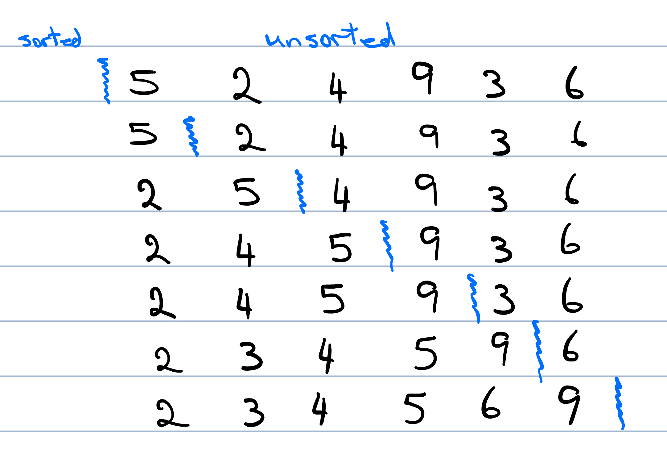
Figure 3.1: Insertion Sort
Since arrays do not allow us to directly insert a value at an arbitrary index, we start from the right-hand side of the sorted section. We compare the element we want to insert (the key) with the elements in the sorted section. If an element in the sorted section is greater than the target, it should be to the right of the target, so we shift it one position to the right. We continue this process until we find an element in the sorted section that is smaller than the target, indicating the correct position for the target. At this point, we insert the target into its correct position in the sorted section. This is demonstrated in Figure 3.1, where we compare 3 and 9 (\(3 < 9 \Rightarrow\) swap), 3 with 5 (\(3 < 5 \Rightarrow\) swap), 3 with 4 (\(3 < 4 \Rightarrow\) swap), and 3 with 2 (\(3 \nless 2 \Rightarrow\) done). We perform three swaps, and when we find that the number to the left of 3 is less than it, then we know that it is in the correct place and that iteration of the loop is finished.
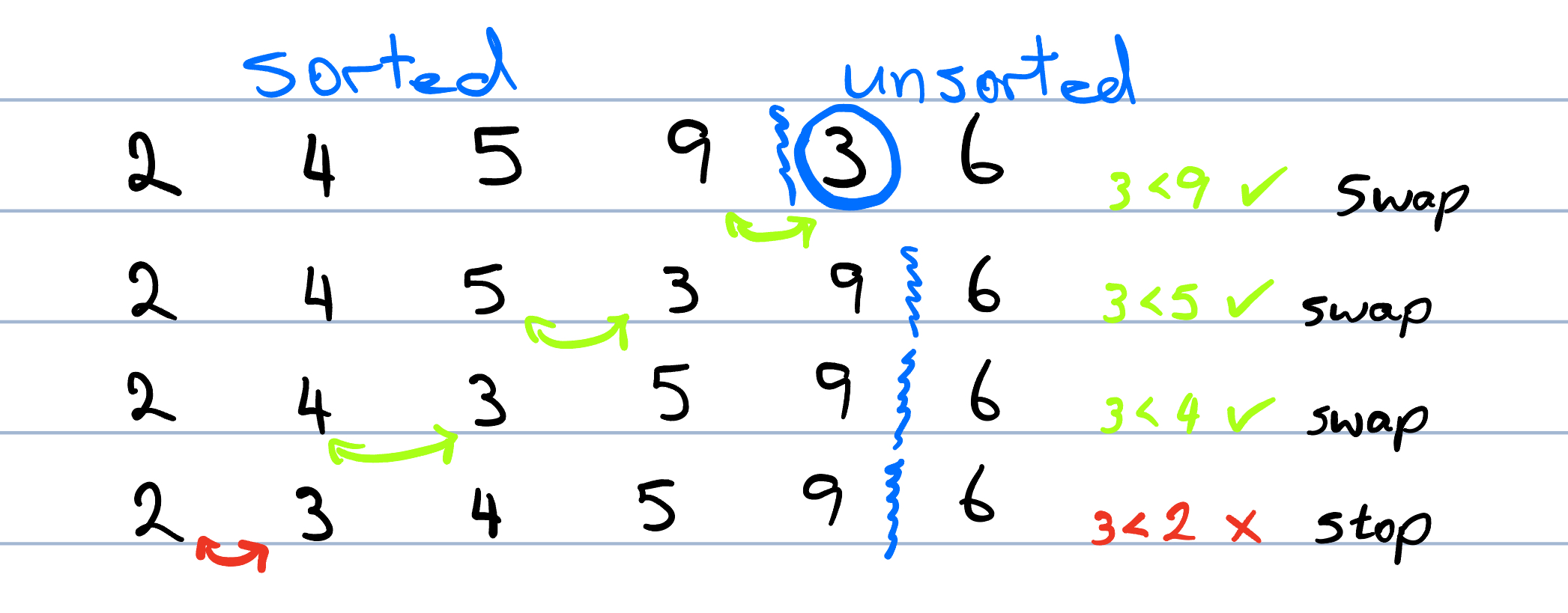
Figure 3.2: Finding the correct position for 3
We repeat this process \(n\) times until we have taken each number out of the unsorted section and inserted it into the sorted section.
3.3.1.1 Pseudocode
InsertionSort(array):
    for i from 1 to length(array):
        j = i - 1
        while j >= 0 and array[j+1] < array[j]:
            swap(array[j+1], array[j])
            j = j - 1
3.3.1.2 Computational Complexity
In our analysis, we will count the number of ‘key comparisons’ (each time we compare two values in the list) and ‘swaps’ (when we see that two values are in the incorrect order).
The best case occurs when we compare the key with a number in the sorted section, and find that they are already in the correct order. When this happens for the first comparison each time, then we never actually enter the inner while loop and our insertion completes immediately. In this case, we do one key comparison and zero swaps per insertion.
This will happen for every iteration when the list is already sorted. For example, in Figure 3.3, we see that we do exactly \(n-1\) comparsions and \(0\) swaps. We never go into the inner loop, so overall, the number of operations that we perform will be \(O(n)\) – linear.
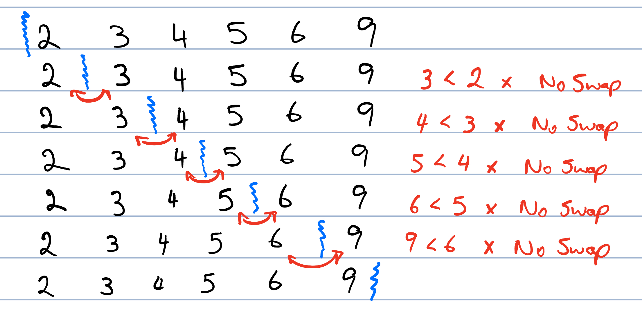
Figure 3.3: Best Case Insertion Sort
The worst case occurs when every key comparison finds that the numbers are in the incorrect order. This happens when the list is sorted in the reverse order. So each time we insert a number into the sorted section, we have to move it all the way to the beginning of the list. This happens at every iteration of the outer for loop.
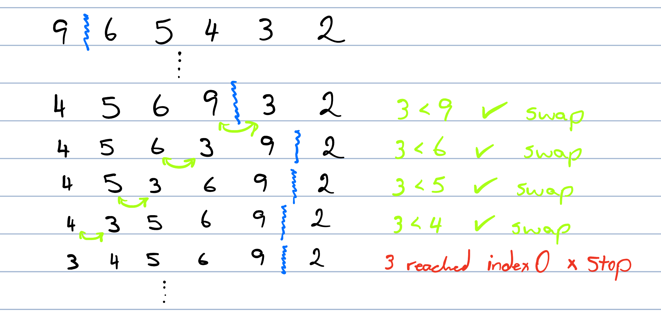
Figure 3.4: Worst Case Insertion Sort
To calculate the number of operations, consider the case where there are \(i\) numbers in the sorted section of the list. The worst case happens when we compare the key to every one of these values (i.e. we do \(i\) comparisons) and each time we see that the values are in the wrong order and perform a swap (i.e. we do \(i\) swaps). We know that the sorted list starts off empty (\(i=0\)) and before the very last iteration of the loop it has all but one of the values in it (\(i = n-1\)). The total amount of work that we will do will be the sum of the work from each main step (i.e. each value of \(i \in \{0,1,2,\ldots, n-1\}\)). From above, we saw that we do \(i-1\) comparisons and \(i-1\) swaps at each step.
Therefore, \[ \mathrm{TotalTime} = a\cdot\mathrm{TotalComparisons} + b\cdot\mathrm{TotalSwaps},\] where \(a\) is the amount of time it takes to do a comparison, and \(b\) is the amount of time it takes to complete a swap, and \[\begin{eqnarray} \mathrm{TotalComparisons} & = & \sum_{i=0}^{n-1} i, \\ \mathrm{TotalSwaps} & = & \sum_{i=0}^{n-1} i. \end{eqnarray}\]
Using the formula for the sum of the first \(n\) integers, \(\sum_{i=0}^n i = \frac{n(n+1)}{2}\), the total amount of work becomes: \[\begin{eqnarray} \mathrm{TotalWork} & = & a\cdot\sum_{i=0}^{n-1} i + b\cdot\sum_{i=0}^{n-1} i \\ & = & (a+b)\cdot\sum_{i=0}^{n-1} i \\ & = & (a+b)\cdot \frac{(n-1)n}{2}\\ & = & (a+b)\cdot \left(\frac{n^2}{2} - \frac{n}{2}\right)\\ & = & O(n^2) \end{eqnarray}\]
So in the worst case, we see that we end up doing a quadratic amount of work: \(O(n^2)\).
- Best Case: \(O(n)\) (list is already sorted)
- Average Case: \(O(n^2)\)
- Worst Case: \(O(n^2)\) (list is reverse sorted)
3.3.2 Selection Sort
Selection Sort is an in-place comparison sorting algorithm. It works by repeatedly selecting the smallest (or largest, depending on the sorting order) element from the unsorted section and moving it to the end of the sorted section. Like Insertion Sort, it is not suitable for large datasets as its average and worst-case complexities are quite high.
We conceptualize the list as being divided into a sorted and an unsorted section. The algorithm iteratively selects the smallest element from the unsorted section and swaps it with the first element in the unsorted section, effectively growing the sorted section by one element and shrinking the unsorted section by one element with each iteration.
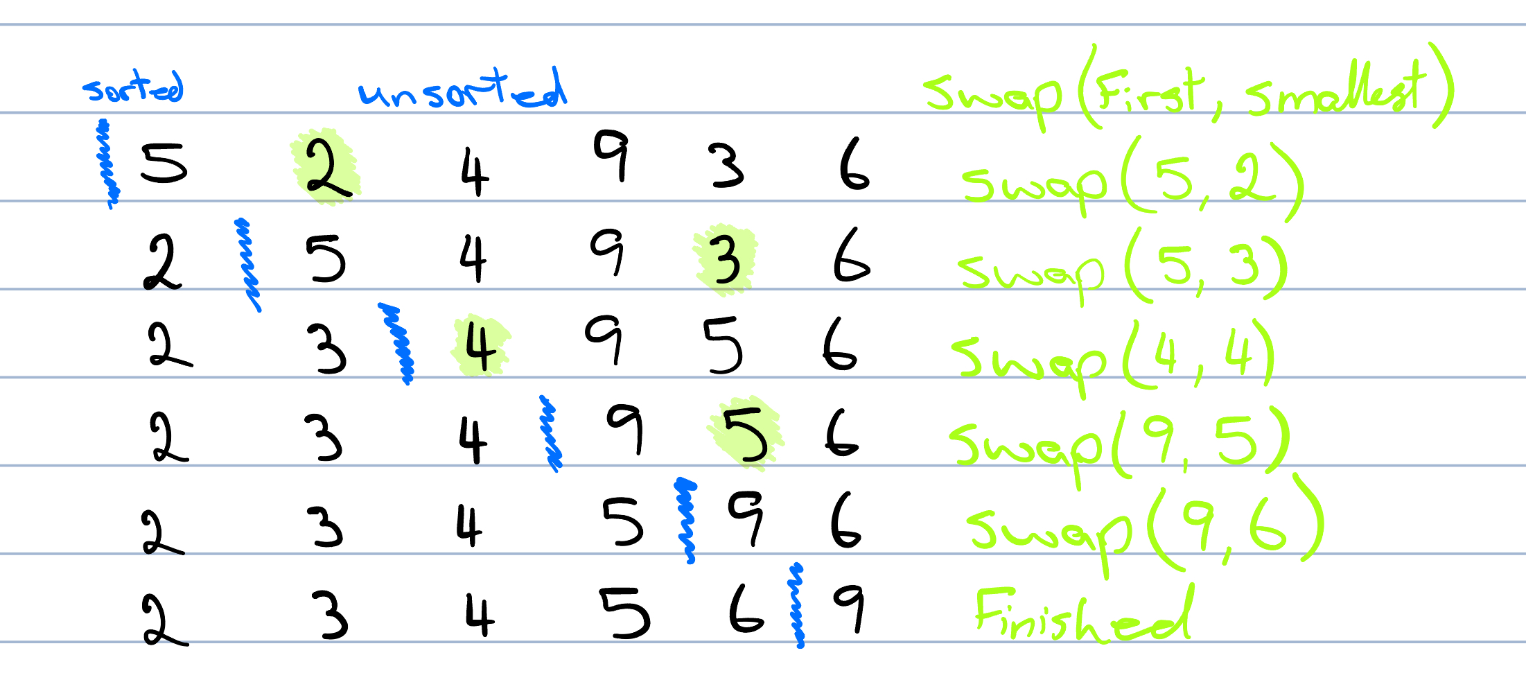
Figure 3.5: Selection Sort
We start from the left-hand side of the unsorted section. We compare each element to find the smallest one. Once we find it, we swap it with the first element in the unsorted section. This process is repeated until the entire list is sorted.
For example, in Figure 3.5, we start with the first element 5 and compare it with all other elements. The smallest element found is 2, so we swap 5 with 2. The list then looks like [2, 5, 4, 9, 3, 6]. The sorted section is now [2] and the unsorted section is [5, 4, 9, 3, 6]. This process is repeated until the entire list is sorted. We repeat this process \(n\) times until the unsorted section is empty and the entire list is sorted.
3.3.2.1 Pseudocode:
SelectionSort(array):
    for i from 0 to length(array) - 1:
        min_index = i
        for j from i + 1 to length(array):
            if array[j] < array[min_index]:
                min_index = j
        swap(array[i], array[min_index])
3.3.2.2 Computational Complexity:
The best, average, and worst cases of Selection Sort all have the same time complexity. Due to the nature of the algorithm; it always performs the same number of comparisons regardless of the initial ordering of the elements.
For each iteration of the algorithm, we need to find the smallest number in the unsorted section of the list. This requires that we look at every number in the remaining unsorted list regardless of the order. So in the first iteration the unsorted section is \(n\) numbers and we must do \(n-1\) comparisons to find the smallest value. The unsorted section is now one value smaller and we need to do \(n-2\) comparisons to find the smallest value. This process continue until eventually there are \(2\) elements in the unsorted list and we need to do \(1\) comparison to figure out which is the smallest.
Therefore, the total number of comparisons is:
\[ (n-1) + (n-2) + \ldots + 1 = \sum_{i=1}^{n-1} i = \frac{(n-1)n}{2} \]
The number of swaps is at most \(n-1\) because each element is swapped at most once.
Using the formula for the sum of the first \(n-1\) integers, the total number of operations is:
\[ \mathrm{TotalTime} = a \cdot \mathrm{TotalComparisons} + b \cdot \mathrm{TotalSwaps}, \]
where \(a\) is the amount of time it takes to do a comparison, and \(b\) is the amount of time it takes to complete a swap.
\[\begin{eqnarray} \mathrm{TotalComparisons} & = & \sum_{i=1}^{n-1} i = \frac{n(n-1)}{2}, \\ \mathrm{TotalSwaps} & = & n-1. \end{eqnarray}\]
The total amount of work becomes:
\[\begin{eqnarray} \mathrm{TotalWork} & = & a \cdot \frac{n(n-1)}{2} + b \cdot (n-1) \\ & = & \frac{a \cdot n^2 - a \cdot n}{2} + b \cdot n - b \\ & = & O(n^2). \end{eqnarray}\]
Thus, the time complexity for Selection Sort is:
- Best Case: \(O(n^2)\)
- Average Case: \(O(n^2)\)
- Worst Case: \(O(n^2)\)
3.3.3 Bubble Sort
Bubble Sort is a simple comparison-based sorting algorithm that repeatedly steps through the list, compares adjacent elements, and swaps them if they are in the wrong order. This process is repeated until the list is sorted. Despite its simplicity, Bubble Sort is not efficient for large lists and is generally outperformed by more advanced algorithms.
The algorithm works by repeatedly “bubbling” the largest unsorted element to the end of the unsorted section of the list. After each full pass through the list, the next largest element is guaranteed to be in its correct position.
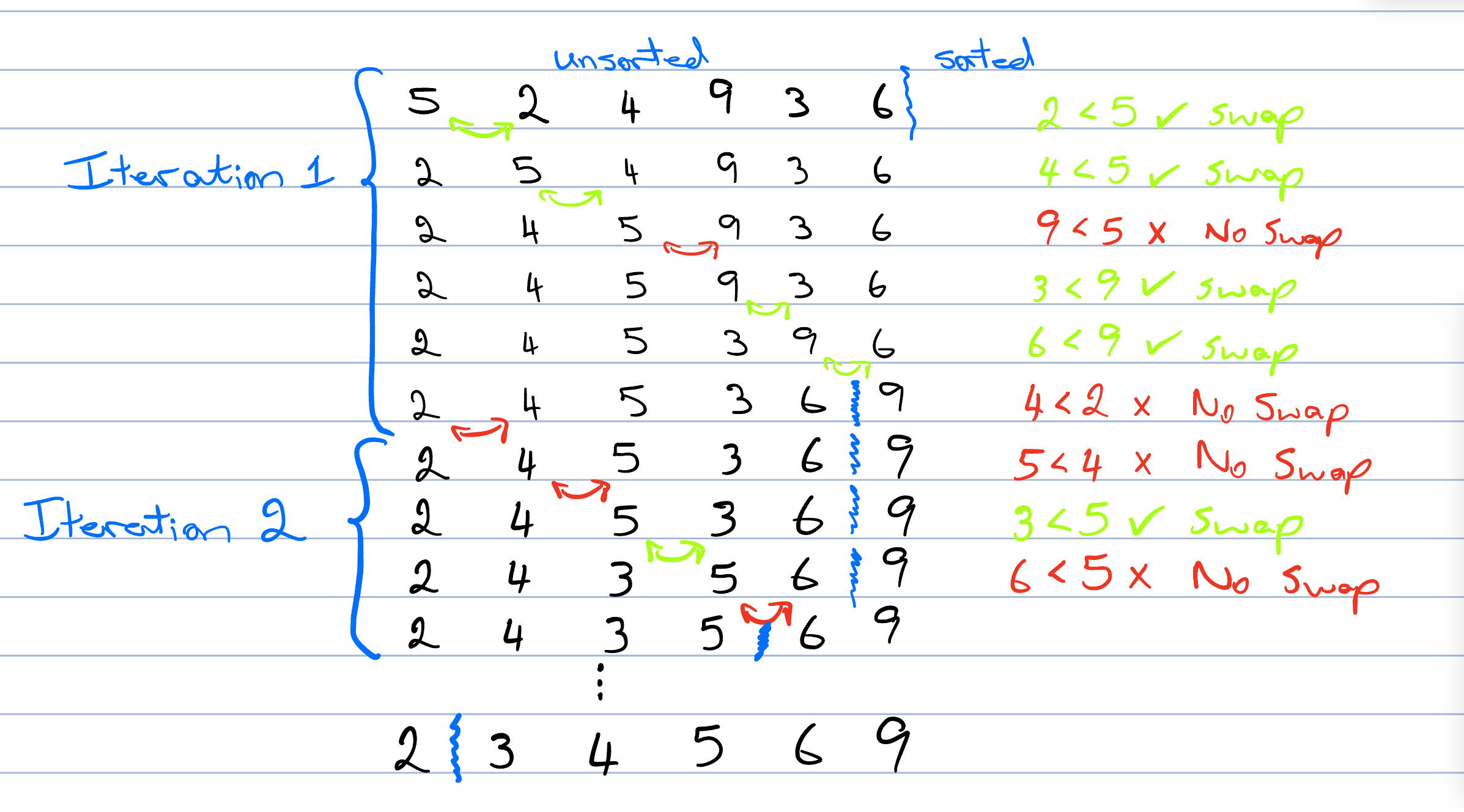
Figure 3.6: Bubble Sort
We start at the beginning of the list and compare the first two elements. If they are in the wrong order, we swap them. We then move one position to the right and repeat this process for each pair of adjacent elements, ending with the last element in the list. After one complete pass, the largest element will be at the end of the list. We then repeat the process for the remaining unsorted section of the list.
For example, in Figure 3.6, we start with the list [5, 2, 4, 9, 3, 6]. We compare 5 and 2 and swap them since 5 > 2. The list becomes [2, 5, 4, 9, 3, 6]. We then compare 5 and 4 and swap them, resulting in [2, 4, 5, 9, 3, 6]. We continue this process until the largest element 9 is bubbled to the end of the list.
We repeat this process \(n\) times until the entire list is sorted.
3.3.3.1 Pseudocode
BubbleSort(array):
    n = length(array)
    for i from 0 to n - 1:
        for j from 0 to n - i - 1:
            if array[j] > array[j + 1]:
                swap(array[j], array[j + 1])
We can add an optimisation to the algorithm that checks whether a swap was made during each iteration. If we ever perform an entire iteration without any swaps, then we know the list is sorted and the algorithm can terminate early.
BubbleSort(array):
    n = length(array)
    for i from 0 to n - 1:
        n_swaps = 0
        for j from 0 to n - i - 1:
            if array[j] > array[j + 1]:
                swap(array[j], array[j + 1])
                n_swaps++
        if n_swaps == 0:
            return
3.3.3.2 Computational Complexity:
The best and worst cases of Bubble Sort all have distinct time complexities.
In the best case, the list is already sorted, so we only need one pass to verify that no swaps are needed. This means that we will have completed \(n-1\) comparisons and \(0\) swaps. We therefore have a time complexity of \(O(n)\) in the best case.
In the worst case, the list is sorted in reverse order, requiring the maximum number of swaps and comparisons. To analyze the complexity, consider that for each element in the list, we need to compare and potentially swap adjacent elements. This requires \(n-1\) comparisons for the first pass, \(n-2\) comparisons for the second pass, and so on, down to \(1\) comparison for the last pass.
Therefore, the total number of comparisons is:
\[ (n-1) + (n-2) + \ldots + 1 = \sum_{i=1}^{n-1} i = \frac{n(n-1)}{2} \]
The number of swaps can vary. In the worst case, each comparison results in a swap, leading to:
\[ (n-1) + (n-2) + \ldots + 1 = \sum_{i=1}^{n-1} i = \frac{n(n-1)}{2} \]
The total time of the algorithm is then:
\[ \mathrm{TotalTime} = a \cdot \mathrm{TotalComparisons} + b \cdot \mathrm{TotalSwaps}, \]
where \(a\) is the amount of time it takes to do a comparison, and \(b\) is the amount of time it takes to complete a swap.
\[\begin{eqnarray} \mathrm{TotalComparisons} & = & \sum_{i=1}^{n-1} i = \frac{n(n-1)}{2}, \\ \mathrm{TotalSwaps} & = & \frac{n(n-1)}{2}. \end{eqnarray}\]
The total amount of work becomes:
\[\begin{eqnarray} \mathrm{TotalWork} & = & a \cdot \frac{n(n-1)}{2} + b \cdot \frac{n(n-1)}{2} \\ & = & (a+b) \cdot \frac{n(n-1)}{2} \\ & = & (a+b) \cdot \left(\frac{n^2}{2} - \frac{n}{2}\right) \\ & = & O(n^2) \end{eqnarray}\]
Thus, the time complexity for Bubble Sort is:
- Best Case: \(O(n)\) (list is already sorted)
- Average Case: \(O(n^2)\)
- Worst Case: \(O(n^2)\) (list is reverse sorted)
3.4 Lab
In this lab (and in many of those that follow) you are given the declaration of a Thing class. This class will always store an integer value, but will usually add in some extra functionality that we can use to help with grading.
class Thing{
public:
    // Stores an integer value
    int i;

    // Constructors
    Thing();
    Thing(int i);
    // Destructor
    ~Thing();

    // Override the comparison operators so that we can print
    //  each time that two Things are compared.
    bool operator==(const Thing& other) const;
    bool operator!=(const Thing& other) const;
    bool operator<(const Thing& other) const;
    bool operator>(const Thing& other) const;
    bool operator<=(const Thing& other) const;
    bool operator>=(const Thing& other) const;

    // A static variable is shared between all instance of an object.
    // You can turn on/off the comparison printing by setting:
    //    Thing::verbose = true // Thing::verbose = false
    static bool verbose;
};
In this lab, the Thing class has an integer (i) and some operator functions that run when we compare two objects. For example:
This will output:
Comparing 5 and 8
Comparing 5 and 42
The following comparison operators can be used: <, <=, ==, !=, >=, >.
There is also a valid print_vector function in main.cpp that iterates through each Thing in the vector and prints out the value.
The provided main function is correct and reads in a list of numbers terminated by -1 followed by a string command. It builds a vector<Thing> containing Thing objects that store the relevant numbers. The following commands will then call the functions that you need to implement:
LinearSearch N- Perform a linear search for the number
Nand output the first index where the value is found. If the value is not in the list, then you should return-1. - Input:
15 38 30 51 33 9 45 24 -1 LinearSearch 45- Output:
15 38 30 51 33 9 45 24 Comparing 15 and 45 Comparing 38 and 45 Comparing 30 and 45 Comparing 45 and 51 Comparing 33 and 45 Comparing 9 and 45 Comparing 45 and 45 Index: 6- Perform a linear search for the number
BinarySearch N- Perform a binary search for the number
Nand output the index where the value is found. If the value is not in the list, then you should return-1. You can assume that the given list will already be sorted and that the numbers in the list are unique. - Input:
9 15 24 30 33 38 45 51 -1 BinarySearch 45- Output:
9 15 24 30 33 38 45 51 Comparing 30 and 45 Comparing 30 and 45 Comparing 38 and 45 Comparing 38 and 45 Comparing 45 and 45 Index: 6- Perform a binary search for the number
InsertionSort- Perform an Insertion Sort on the provided list. You should output the state of the list after each iteration of the outer loop (i.e. after each insertion step). The function should return the sorted vector.
- Input:
30 51 15 24 45 38 9 33 -1 InsertionSort- Output:
30 51 15 24 45 38 9 33 Comparing 30 and 51 30 51 15 24 45 38 9 33 Comparing 15 and 51 Comparing 15 and 30 15 30 51 24 45 38 9 33 Comparing 24 and 51 Comparing 24 and 30 Comparing 15 and 24 15 24 30 51 45 38 9 33 Comparing 45 and 51 Comparing 30 and 45 15 24 30 45 51 38 9 33 Comparing 38 and 51 Comparing 38 and 45 Comparing 30 and 38 15 24 30 38 45 51 9 33 Comparing 9 and 51 Comparing 9 and 45 Comparing 9 and 38 Comparing 9 and 30 Comparing 9 and 24 Comparing 9 and 15 9 15 24 30 38 45 51 33 Comparing 33 and 51 Comparing 33 and 45 Comparing 33 and 38 Comparing 30 and 33 9 15 24 30 33 38 45 51SelectionSort- Perform a Selection Sort on the provided list. You should output the state of the list after each iteration of the outer loop (i.e. after the minimum value is swaped in). The function should return the sorted vector.
- Input:
30 51 15 24 45 38 9 33 -1 SelectionSort- Output:
30 51 15 24 45 38 9 33 Comparing 30 and 51 Comparing 15 and 30 Comparing 15 and 24 Comparing 15 and 45 Comparing 15 and 38 Comparing 9 and 15 Comparing 9 and 33 9 51 15 24 45 38 30 33 Comparing 15 and 51 Comparing 15 and 24 Comparing 15 and 45 Comparing 15 and 38 Comparing 15 and 30 Comparing 15 and 33 9 15 51 24 45 38 30 33 Comparing 24 and 51 Comparing 24 and 45 Comparing 24 and 38 Comparing 24 and 30 Comparing 24 and 33 9 15 24 51 45 38 30 33 Comparing 45 and 51 Comparing 38 and 45 Comparing 30 and 38 Comparing 30 and 33 9 15 24 30 45 38 51 33 Comparing 38 and 45 Comparing 38 and 51 Comparing 33 and 38 9 15 24 30 33 38 51 45 Comparing 38 and 51 Comparing 38 and 45 9 15 24 30 33 38 51 45 Comparing 45 and 51 9 15 24 30 33 38 45 51BubbleSort- Perform a Bubble Sort on the provided list. You should output the state of the list after each iteration of the outer loop (i.e. when the next largest number has been pulled to the back of the unsorted section). The function should return the sorted vector. You should implement the optimization so that the function returns immediately if no swaps are made in an iteration.
- Input:
30 51 15 24 45 38 9 33 -1 BubbleSort- Output:
30 51 15 24 45 38 9 33
Comparing 30 and 51
Comparing 15 and 51
Comparing 24 and 51
Comparing 45 and 51
Comparing 38 and 51
Comparing 9 and 51
Comparing 33 and 51
30 15 24 45 38 9 33 51
Comparing 15 and 30
Comparing 24 and 30
Comparing 30 and 45
Comparing 38 and 45
Comparing 9 and 45
Comparing 33 and 45
15 24 30 38 9 33 45 51
Comparing 15 and 24
Comparing 24 and 30
Comparing 30 and 38
Comparing 9 and 38
Comparing 33 and 38
15 24 30 9 33 38 45 51
Comparing 15 and 24
Comparing 24 and 30
Comparing 9 and 30
Comparing 30 and 33
15 24 9 30 33 38 45 51
Comparing 15 and 24
Comparing 9 and 24
Comparing 24 and 30
15 9 24 30 33 38 45 51
Comparing 9 and 15
Comparing 15 and 24
9 15 24 30 33 38 45 51
Comparing 9 and 15
9 15 24 30 33 38 45 51
The output should include the required list printouts as mentioned above, as well as printouts from each Thing comparison that is made. So to pass a test case, you do need to be performing the comparisons in the correct order.
The marker uses IO tests so your output should match that of the sample input/output. You can download some more sample test cases and the project files here.