Chapter 13 Recursion

One of the most powerful concepts in computer science and programming is that of recursion. Wikipedia has a great definition of recursion: recursion occurs when a thing is defined in terms of itself. This is particularly useful to us when the solution to a problem depends on smaller instances of the same problem. For example, playing chess can be defined recursively: assume that we have a function called playChess that is able to play a game of chess by picking good moves. This function can be defined recursively as: play a move, then execute playChess from the resulting position! Since playChess calls the function playChess, it is said to be a recursive function.

13.1 Computing the factorial

There is an equivalence between iteration and recursion—anything that can be done with a loop can be done with recursion, and vice versa. We can think of iteration as counting up, and recursion as counting down. To see this, consider the canonical example of the factorial function (\(!\)). Factorial is a mathematical function where:

\[N! = 1 \times 2 \times \ldots \times (N - 1) \times N.\]

By definition, we also have \(0! = 1\).

From the above, it is clear that we can write the factorial function as a recursive function of any non-negative integer as follows:

\[N! = \begin{cases} 1 \text{ if } N = 0 \\ N \times (N - 1)! \text{ otherwise.} \end{cases}\]

Note that the above definition of the factorial is recursive, since the right-hand-side of the definition itself contains a factorial function. Bot approaches are equivalent to one another—they will both successfully compute the factorial of a number. However, the first approach is iterative; it shows how to compute the factorial by multiplying all the numbers from \(1\) up to \(N\). By contrast, the second approach is recursive. As we mentioned, there is an equivalence between iteration and recursion, and so the choice depends on whether it is easier to model the problem recursively or iteratively. We now present the C++ functions for the two equations above:

int factorialIterative(int N){
    int factorial = 1;
    for (int i = 1; i <= N; ++i){
        factorial *= i  
    }   
    return factorial;   
}

int factorialRecursive(int N){
    if (N == 0){
        return 1;  //this is the base case  
    }
    return N * factorialRecursive(N - 1)
}

Notice that the recursive definition has what we call a base case. This is also known as an escape hatch, and is equivalent to a loop’s terminating condition. It is a non-recursive statement that breaks the chain of recursion. Without it, we would have infinite recursion (which is the equivalent of an infinite loop). To see this, imagine we left out the base case:

int factorialBad(int N){
    return N * factorialBad(N - 1)
}

Without the base case, the above is equivalent to \(N \times (N-1) \times (N-2) \times (N-3) \times (N-4) \times \ldots\) forever. The base case breaks this chain, so that when we reach zero, it stops.

In order to understand exactly what happens behind the scene, we must first discuss the concept of a stack frame. Before that, a final note on the difference between recursion and iteration. In general, recursion is often more readable and intuitive that iteration. Its main downside is that it is often slower and uses more memory. However, one major advantage is that, unlike iteration, it does not require mutable state. Mutable state refers to the fact that we have variables that can change their value. For iteration, the loop counter is a mutable object. In general, the more things that change, the more that can go wrong. Recursion is a way to achieve the same result, without the need for mutable variables, and so is a very powerful tool.⁴

Programming language side quest! The standard tradeoff between recursive and iterative solutions is that iteration is faster, but harder to code and reason about, whereas recursion is easier to think about, but also slower to execute and can quickly run into memory issues. However, certain languages support the concept of tail recursion, which is a form of recursion that has all the benefits of iteration and recursion wrapped into one! First, use Google to learn about tail recursion. Then, rewrite the factorial code above to take advantage of tail call optimisation. Finally, if you have a relatively modern C++ compiler, try follow this tutorial to see what’s happening behind the scenes!

13.2 The stack frame

C++ programs and the variables and functions they declare are all stored in memory. The memory that the program is allocated is divided into the following sections:

Figure 13.1: Memory allocated to the program divided into sections

1. The code section is where the entire program (with all its instructions compiled to machine language) is stored.

2. Static data is where global variables are stored

3. The heap is a collection of extra memory that is assigned to us. We will look at the heap in more detail in the next chapter

4. The stack is where local variables reside.

Variables in the stack have automatic allocation. This means that when we declare a local variable, the compiler automatically finds an appropriate memory location for it. Similarly, when the variables go out of scope, the compiler automatically frees that memory.

The stack consists of a series of frames called stack frames. Stack frames are stacked on top of the other (hence the name), and only the top-most one is “visible” to the program. Every time a function is called, a new stack frame is placed on the stack. Each stack frame stores the arguments passed to that function, the local variables declared in the function, the state of the CPU at that time, and the return address (that is, which line should be next executed after the function returns?) When a function ends, its stack frame is discarded from the stack. This “reveals” the stack frame underneath it.

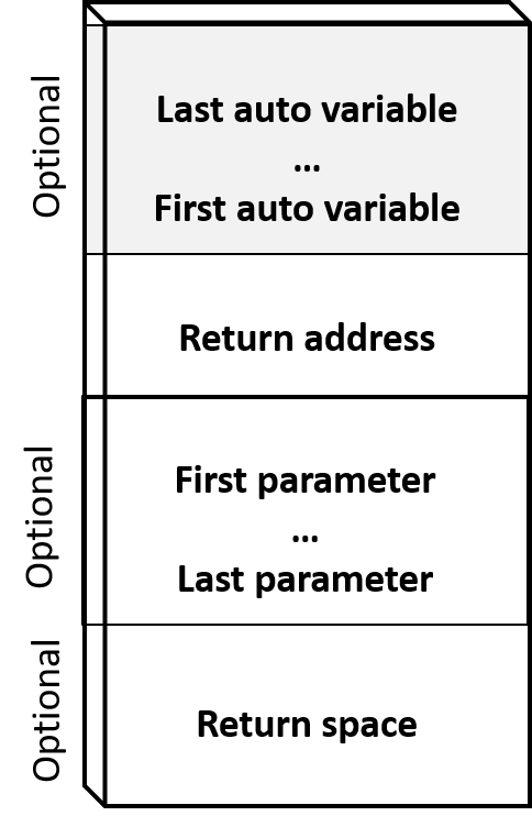
Figure 13.2: A single stack frame, which holds the local variables, the return address, the function’s parameters and space for the value being returned (if any).

We can think of stack frames as the variables that the program is currently working with. If a variable exists in a stack frame that is not on top, then it cannot currently be referenced. This is how the scope of variables is managed.

We will first look at how this works with a single function call, before moving on to the recursive case. The code below has two functions. We will show how stack frames are added and removed as we proceed through the code one line at a time. The arrows on the left indicate which line we are currently executing.

#include <iostream>

using namespace std;

int square(int x){
    int y = x * x;
    cout << y << endl;
    return y;
}

int main(){
    int x = 2;
    int z = square(x);
    return 0;
}

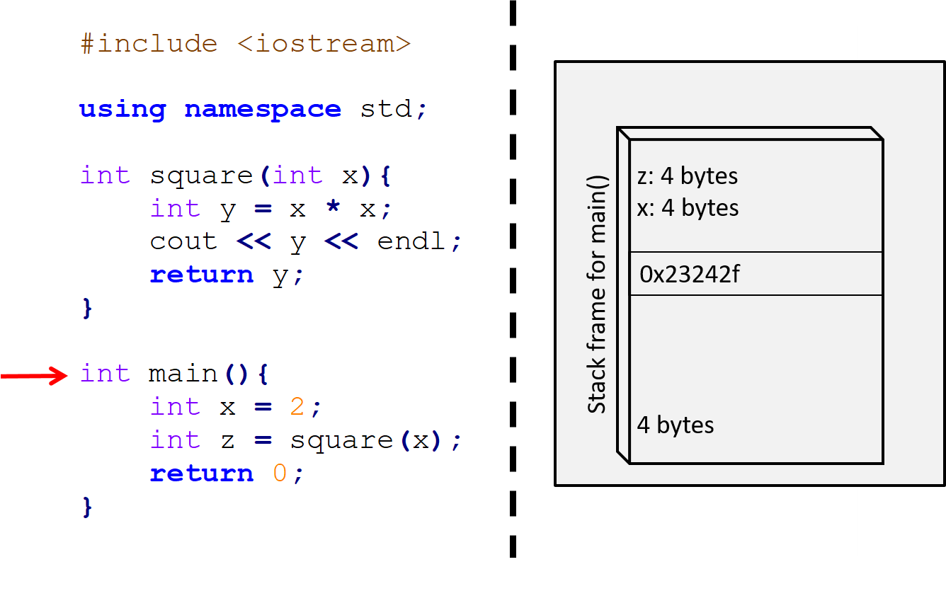
Figure 13.3: We begin inside the main function, and so there is a single stack frame on the stack belonging to main. The function has two local variables, x and z, which are stored in its stack frame. It also returns an integer, and so its return space is 4 bytes wide.

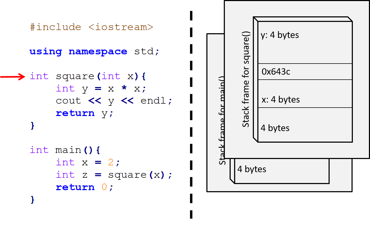
Figure 13.4: We then call the square function, which has a single parameter x and local variable y. It also returns an integer and so have 4 bytes allocated for this. Its stack frame is now placed on the stack on top of main’s. Thus at this point, the variables in main’s stack frame cannot be accessed.

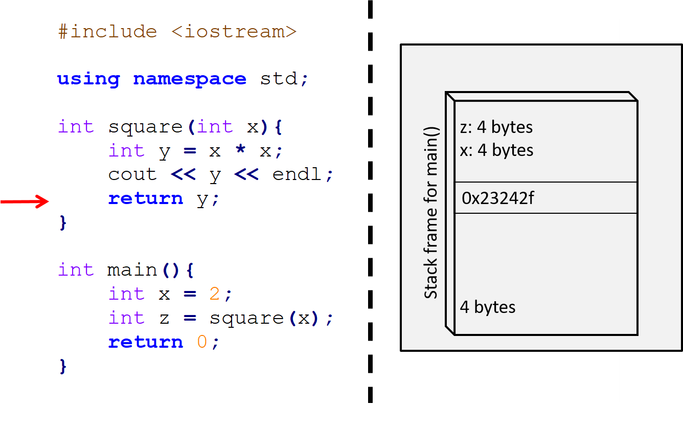
Figure 13.5: Finally, on Line 8, the square function returns. Its return value is stored in an appropriate place, and its stack frame is discarded, leaving once again only main’s stack frame left.

A similar procedure occurs when we use a recursive function, although the number of stack frames added to the stack depends on how many recursive calls occur.⁵ We will illustrate what happens when the factorial function below is called with \(N = 3\).

int factorial(int N){
    if (N == 0){
        return 1; 
    }
    return N * factorial(N - 1)
}

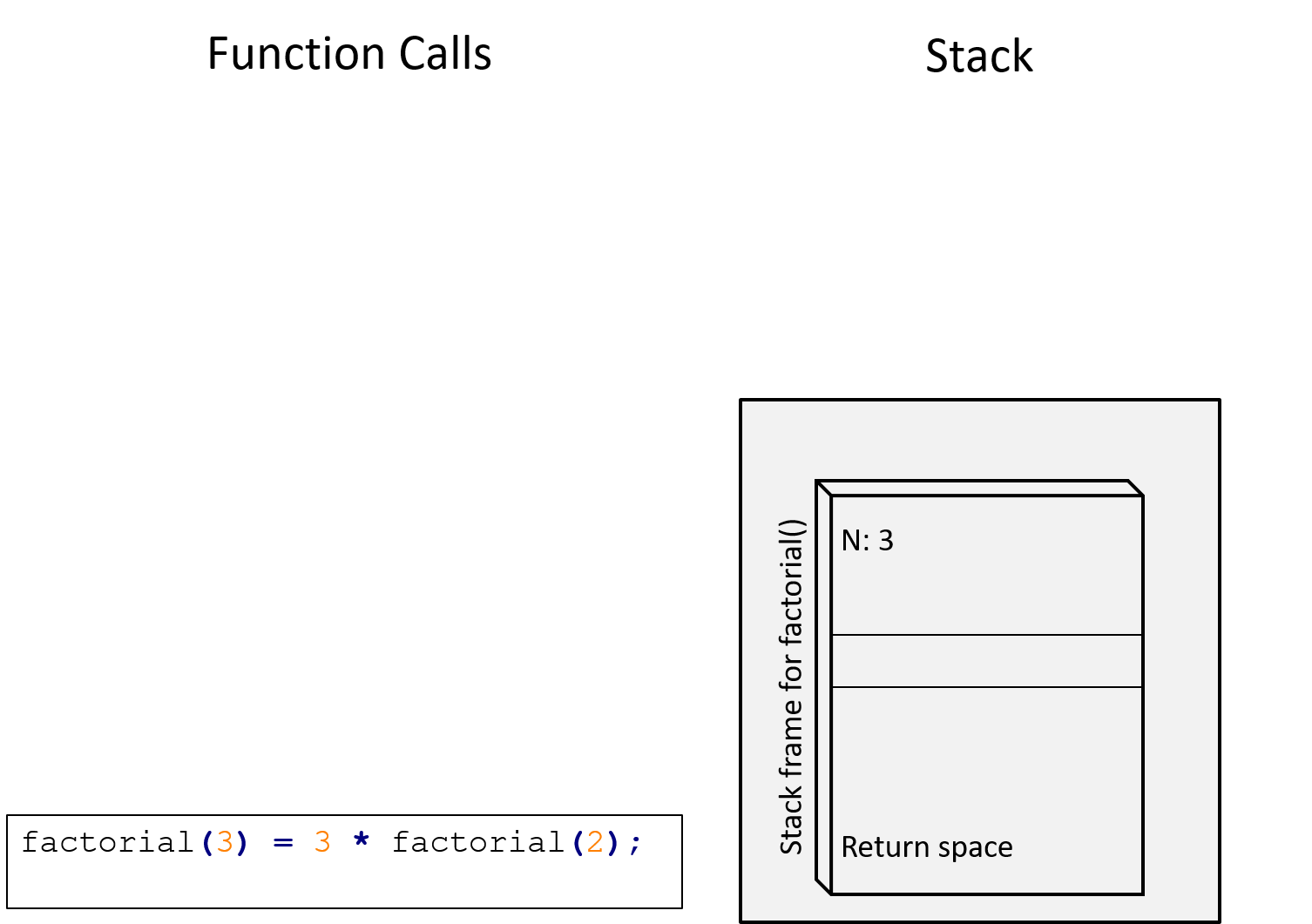
Figure 13.6: We first invoke factorial(3). Hence there is a single frame on the stack. The function will then proceed to compute \(3 imes\)factorial(2)

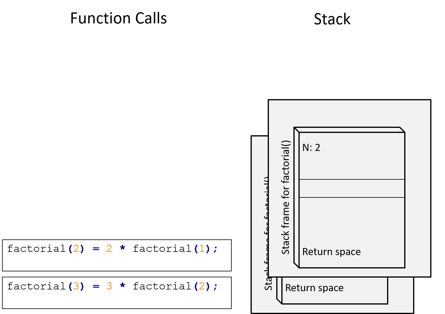
Figure 13.7: factorial(2) has just been called, adding a stack frame on top of the previous one. The function will then proceed to compute \(2 imes\) factorial(1)

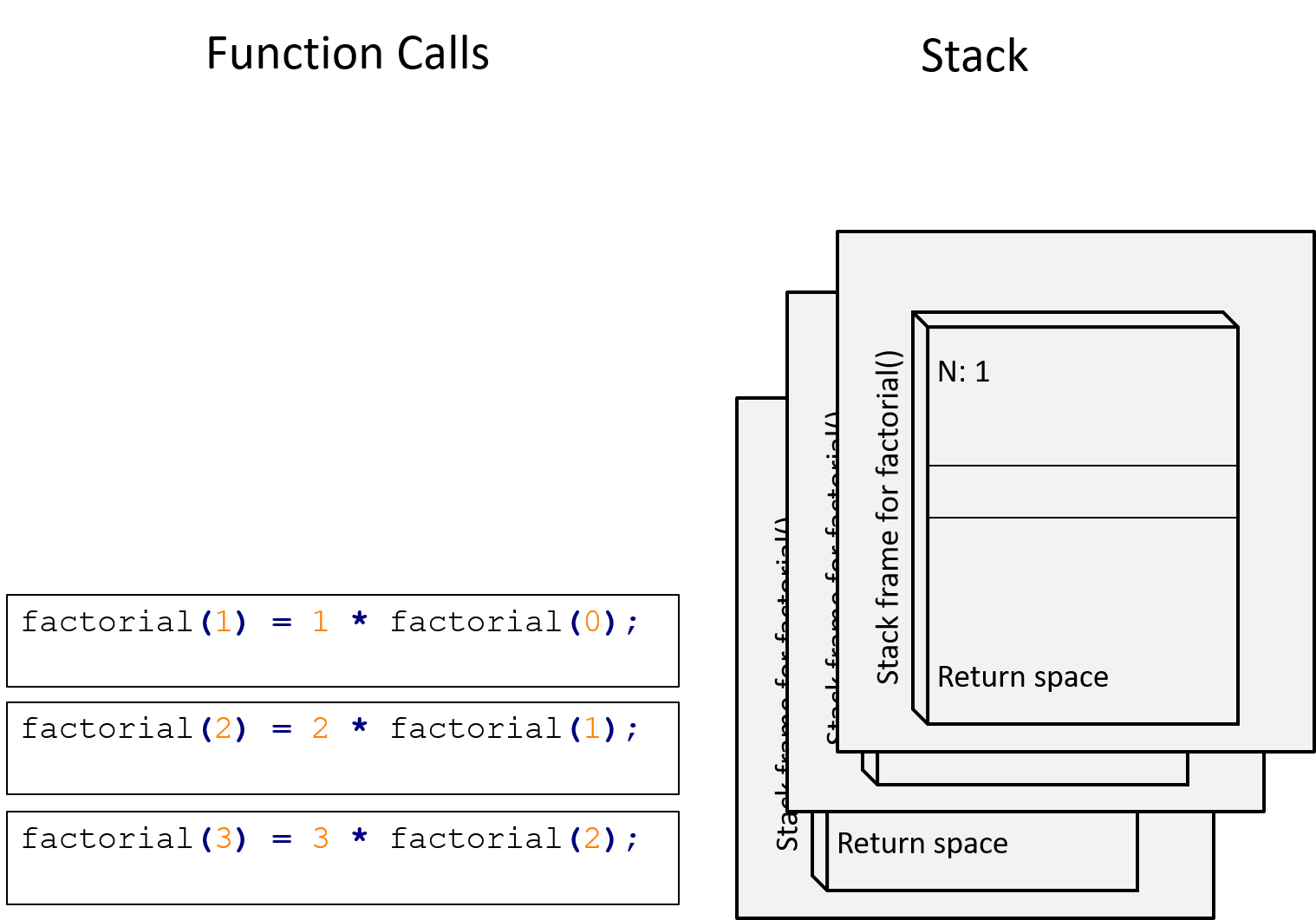
Figure 13.8: factorial(1) has just been called, adding a third stack frame. The function will then proceed to compute \(1 imes\) factorial(0)

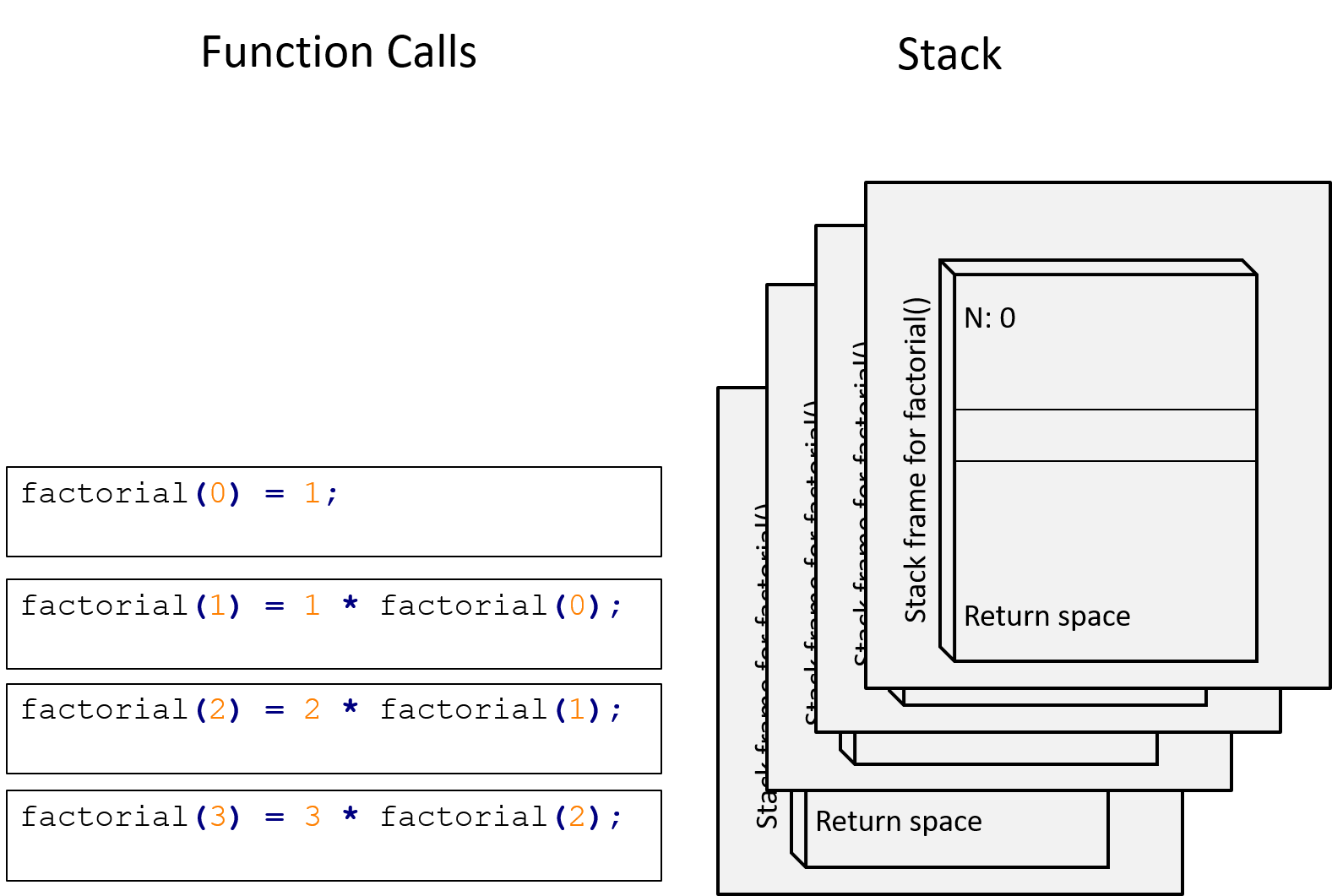
Figure 13.9: factorial(0) has just been called, adding a fourth stack frame. The function will then proceed to return \(1\). No more recursive calls are made, and so the top stack frame will be removed.

Now that the base case has been reached, the stack starts to unwind. The frame for factorial(0) is removed, and the value \(1\) is returned. Then, factorial(1) can compute its return value as \(1 \times 1\). It returns \(1\), and the frame for factorial(1) is removed. Similarly, factorial(2) can compute its return value as \(2 \times 1\). It returns \(2\), and the frame for factorial(2) is removed. Finally, factorial(3) computes \(3 \times 2\). The answer \(6\) is returned and the frame for factorial(3) is removed.

13.3 Summary lecture

Programming side quest! Use the algorithm presented in the above video to create a Sudoku solver program. Your program should be able to read in a partially-completed Sudoku puzzle and output a solution, or an error message if none exists. Bonus quest! Try extend your program to solve \(16 \times 16\) versions!

---

4. This is a very good reason for using pointers. For example, imagine you wrote a function that searches an array and returns a pointer to the element in the array with a particular value. What if there is no such element matching that value? What should we return in that case? A pointer that points to “null” is a good candidate in this case.↩︎

5. The reason it is forbidden is that C++ was initially designed to be backward compatible with its predecessor programming languages B and C. Since these languages do not allow for one array to be assigned to another, neither does C++.↩︎