Appendix D — Recurrent Networks: Details and Implementation
Recurrent neural networks (RNNs) process sequences by iteratively applying a parameterized state update. Where a feedforward layer maps an input vector directly to an output, an RNN maintains a hidden state vector that summarizes historical inputs, updating that state at every step. This appendix formalizes the mathematics of recurrent networks, derives backpropagation through time and its gradient pathologies, details the gating mechanisms in LSTMs and GRUs, and provides a standalone, runnable implementation of a sequence-to-sequence model.
D.1 The vanilla recurrence and tensor shapes
D.1.1 Mathematical formulation and unrolling
Let \(x_t \in \mathbb{R}^{D_{\text{in}}}\) denote the input vector at discrete time step \(t \in \{1, \dots, T\}\), and let \(h_{t-1} \in \mathbb{R}^{D_h}\) denote the hidden state carried over from the preceding position. A standard vanilla recurrent network computes an intermediate affine pre-activation \(a_t\) and passes it through an element-wise saturating nonlinearity (typically the hyperbolic tangent, \(\tanh\)):
\[ a_t = W_{xh} x_t + W_{hh} h_{t-1} + b_h, \qquad h_t = \tanh(a_t), \]
where \(W_{xh} \in \mathbb{R}^{D_h \times D_{\text{in}}}\) is the input-to-hidden weight matrix, \(W_{hh} \in \mathbb{R}^{D_h \times D_h}\) is the recurrent hidden-to-hidden weight matrix, and \(b_h \in \mathbb{R}^{D_h}\) is the bias vector. When a task requires an output at step \(t\), a linear projection produces logits or continuous predictions:
\[ \hat{y}_t = W_{hy} h_t + b_y, \]
with \(W_{hy} \in \mathbb{R}^{D_{\text{out}} \times D_h}\) and \(b_y \in \mathbb{R}^{D_{\text{out}}}\). The initial hidden state \(h_0\) is conventionally set to a vector of zeros, \(h_0 = \mathbf{0}\), though it can also be treated as a learned parameter.
The defining architectural principle of recurrence is parameter sharing through time: the exact same matrices \(\{W_{xh}, W_{hh}, W_{hy}\}\) and biases \(\{b_h, b_y\}\) are applied at step \(1\), step \(2\), and step \(T\). Laying out this recurrent step across time creates an acyclic directed graph of \(T\) sequential stages, a process termed unrolling. While the parameters are identical across steps, the intermediate hidden states \(h_t\) vary dynamically as new inputs arrive.
D.1.2 A small numerical unrolling
To see how parameter sharing and state accumulation interact numerically, consider copying the running digit sequence 4 2 7 from Chapter 7. Let the input at each position be a normalized scalar \(x_t = \text{digit} / 10 \in \mathbb{R}^1\), and let the network maintain a two-dimensional hidden state \(h_t \in \mathbb{R}^2\) with parameters:
\[ W_{xh} = \begin{bmatrix} 0.5 \\ -0.4 \end{bmatrix}, \qquad W_{hh} = \begin{bmatrix} 0.8 & -0.2 \\ 0.1 & 0.7 \end{bmatrix}, \qquad b_h = \begin{bmatrix} 0.1 \\ -0.1 \end{bmatrix}, \qquad h_0 = \begin{bmatrix} 0.0 \\ 0.0 \end{bmatrix}. \]
We trace the step-by-step update:
Step 1 (\(t=1\), input digit
4, \(x_1 = 0.4\)): \[ a_1 = \begin{bmatrix} 0.5(0.4) \\ -0.4(0.4) \end{bmatrix} + \begin{bmatrix} 0.8(0) - 0.2(0) \\ 0.1(0) + 0.7(0) \end{bmatrix} + \begin{bmatrix} 0.1 \\ -0.1 \end{bmatrix} = \begin{bmatrix} 0.2 + 0.1 \\ -0.16 - 0.1 \end{bmatrix} = \begin{bmatrix} +0.3000 \\ -0.2600 \end{bmatrix}. \] Passing through \(\tanh\) gives: \[ h_1 = \begin{bmatrix} \tanh(0.3000) \\ \tanh(-0.2600) \end{bmatrix} = \begin{bmatrix} +0.2913 \\ -0.2543 \end{bmatrix}. \]Step 2 (\(t=2\), input digit
2, \(x_2 = 0.2\)): \[ a_2 = \begin{bmatrix} 0.5(0.2) \\ -0.4(0.2) \end{bmatrix} + \begin{bmatrix} 0.8(0.2913) - 0.2(-0.2543) \\ 0.1(0.2913) + 0.7(-0.2543) \end{bmatrix} + \begin{bmatrix} 0.1 \\ -0.1 \end{bmatrix} = \begin{bmatrix} 0.1 + 0.2839 + 0.1 \\ -0.08 - 0.1489 - 0.1 \end{bmatrix} = \begin{bmatrix} +0.4839 \\ -0.3289 \end{bmatrix}. \] \[ h_2 = \begin{bmatrix} \tanh(0.4839) \\ \tanh(-0.3289) \end{bmatrix} = \begin{bmatrix} +0.4494 \\ -0.3177 \end{bmatrix}. \]Step 3 (\(t=3\), input digit
7, \(x_3 = 0.7\)): \[ a_3 = \begin{bmatrix} 0.5(0.7) \\ -0.4(0.7) \end{bmatrix} + \begin{bmatrix} 0.8(0.4494) - 0.2(-0.3177) \\ 0.1(0.4494) + 0.7(-0.3177) \end{bmatrix} + \begin{bmatrix} 0.1 \\ -0.1 \end{bmatrix} = \begin{bmatrix} 0.35 + 0.4231 + 0.1 \\ -0.28 - 0.1775 - 0.1 \end{bmatrix} = \begin{bmatrix} +0.8731 \\ -0.5575 \end{bmatrix}. \] \[ h_3 = \begin{bmatrix} \tanh(0.8731) \\ \tanh(-0.5575) \end{bmatrix} = \begin{bmatrix} +0.7030 \\ -0.5057 \end{bmatrix}. \]
The final context vector \(c = h_3 = (+0.7030, -0.5057)^\top\) contains the cumulative contribution of all three digits. Even though \(W_{hh}\) and \(W_{xh}\) never changed, the coordinates of \(h_t\) evolved nonlinearly at each step.
D.1.3 Tensor layouts and dimensions
In deep learning frameworks such as PyTorch, recurrent layers operate on batched multidimensional tensors. Two conventions exist for ordering the batch and time axes:
- Batch-first layout (
batch_first=True):- Input tensor \(X\): shape \((B, T, D_{\text{in}})\), where \(B\) is batch size, \(T\) is sequence length, and \(D_{\text{in}}\) is feature dimensionality.
- Intermediate state sequence \(H\): shape \((B, T, D_h)\), concatenating the hidden states across all steps.
- Final hidden state \(h_T\): shape \((B, D_h)\) (or \((1, B, D_h)\) when indexed across multiple RNN layers).
- Time-first layout (
batch_first=False):- Input tensor \(X\): shape \((T, B, D_{\text{in}})\).
- Hidden state sequence \(H\): shape \((T, B, D_h)\).
While time-first ordering was historically preferred because it aligns memory along time slices for recurrent loops in hardware, batch-first is widely adopted in modern pipelines to match standard vision and transformer tensor conventions.
D.1.4 Taxonomy of recurrent sequence configurations
Recurrent networks are versatile because their input and output temporal dimensions can be configured independently. Figure D.1 illustrates the four common arrangements encountered in vision and multimodal learning.
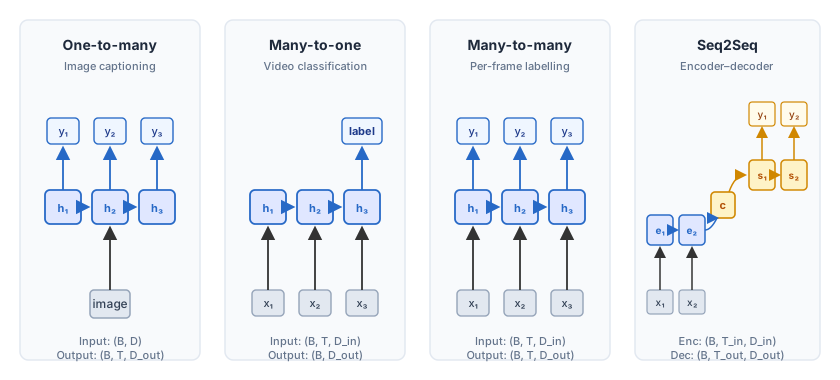
| Arrangement | Input shape | Output shape | Vision application |
|---|---|---|---|
| One-to-many | \((B, D_{\text{in}})\) | \((B, T_{\text{out}}, D_{\text{out}})\) | Image captioning (Show and Tell [1]): a single CNN image embedding seeds an RNN decoder. |
| Many-to-one | \((B, T_{\text{in}}, D_{\text{in}})\) | \((B, D_{\text{out}})\) | Video action recognition: frame embeddings are consumed sequentially; the final state \(h_T\) classifies the clip. |
| Many-to-many (synchronic) | \((B, T, D_{\text{in}})\) | \((B, T, D_{\text{out}})\) | Video object tracking or per-frame action segmentation: each frame \(x_t\) yields an immediate label \(y_t\). |
| Many-to-many (asynchronous / seq2seq) | \((B, T_{\text{in}}, D_{\text{in}})\) | \((B, T_{\text{out}}, D_{\text{out}})\) | Sequence copying, machine translation, or video description: input and output sequences have different lengths. |
The sequence-to-sequence structure (panel d) is central to Chapters 7 and 8: the encoder reads \(T_{\text{in}}\) tokens, compresses them into the single context vector \(c = h_{T_{\text{in}}}\), and hands that vector to the decoder.
D.2 Backpropagation through time
D.2.1 Gradient accumulation across unrolled steps
To train the recurrent parameters \(\{W_{xh}, W_{hh}, b_h, W_{hy}, b_y\}\), we define a scalar training objective. For a sequence of length \(T\) with step losses \(\ell_t = \ell(y_t^*, \hat{y}_t)\), the total sequence loss is:
\[ L = \sum_{t=1}^T \ell_t. \]
Because \(W_{hh}\) is used at every step \(t \in \{1, \dots, T\}\), the multivariable chain rule dictates that the total gradient \(\frac{\partial L}{\partial W_{hh}}\) is the sum of the parameter’s contributions at each individual step:
\[ \frac{\partial L}{\partial W_{hh}} = \sum_{t=1}^T \frac{\partial \ell_t}{\partial W_{hh}}. \]
Focusing on the loss \(\ell_t\) at a single time step \(t\), the hidden state \(h_t\) depends on \(W_{hh}\) both directly (through the current update \(h_t = \tanh(W_{xh} x_t + W_{hh} h_{t-1} + b_h)\)) and indirectly (through all prior states \(h_{t-1}, h_{t-2}, \dots, h_1\)). Expanding this chain of temporal dependencies yields:
\[ \frac{\partial \ell_t}{\partial W_{hh}} = \sum_{k=1}^t \frac{\partial \ell_t}{\partial h_t} \frac{\partial h_t}{\partial h_k} \frac{\partial h_k}{\partial W_{hh}}, \]
where \(\frac{\partial h_k}{\partial W_{hh}}\) denotes the local derivative holding \(h_{k-1}\) fixed. The factor \(\frac{\partial h_t}{\partial h_k}\) is the Jacobian matrix that propagates the error gradient from step \(t\) backward to step \(k\).
D.2.2 Derivation of recurrent Jacobians and gradient stability
By applying the chain rule across the intervening states from \(k\) to \(t\), the temporal Jacobian product decomposes into:
\[ \frac{\partial h_t}{\partial h_k} = \prod_{j=k+1}^t \frac{\partial h_j}{\partial h_{j-1}}. \]
Recalling that \(h_j = \tanh(a_j)\) with \(a_j = W_{xh} x_j + W_{hh} h_{j-1} + b_h\), the single-step Jacobian is:
\[ \frac{\partial h_j}{\partial h_{j-1}} = \operatorname{diag}\bigl(1 - \tanh^2(a_j)\bigr) W_{hh}^\top = D_j W_{hh}^\top, \]
where \(D_j = \operatorname{diag}(1 - h_j^2) \in \mathbb{R}^{D_h \times D_h}\) is a diagonal matrix containing the element-wise derivatives of the \(\tanh\) activation function. Substituting this back into the multi-step Jacobian gives:
\[ \frac{\partial h_t}{\partial h_k} = \prod_{j=k+1}^t D_j W_{hh}^\top = D_t W_{hh}^\top D_{t-1} W_{hh}^\top \cdots D_{k+1} W_{hh}^\top. \]
This product reveals the source of the fundamental training instabilities in recurrent networks:
- Vanishing gradients: The derivative of hyperbolic tangent satisfies \(0 < 1 - \tanh^2(a) \leq 1\). Consequently, the operator norm of each diagonal matrix is bounded: \(\|D_j\|_2 \leq 1\). If the largest singular value of the recurrent weight matrix satisfies \(\sigma_{\max}(W_{hh}) < 1\), then: \[ \left\| \frac{\partial h_t}{\partial h_k} \right\|_2 \leq \prod_{j=k+1}^t \|D_j\|_2 \|W_{hh}^\top\|_2 \leq \bigl(\sigma_{\max}(W_{hh})\bigr)^{t-k}. \] As the temporal separation \(t - k\) grows, the upper bound decays exponentially toward zero. Even if \(\sigma_{\max}(W_{hh}) \approx 1\), whenever the hidden states operate in the saturating regions of \(\tanh\) (\(|a| > 2\)), the entries of \(D_j\) drop substantially below 1, causing the gradient signal to vanish after only 10–20 steps. As a result, parameters cannot be adjusted based on long-range dependencies.
- Exploding gradients: Conversely, if \(\sigma_{\max}(W_{hh}) > 1\) and the network operates in the linear regime of \(\tanh\) (\(a \approx 0\), so \(D_j \approx I\)), the norm can grow as \(\bigl(\sigma_{\max}(W_{hh})\bigr)^{t-k}\). The gradient blows up exponentially, leading to numerical overflow (
NaN), destructive parameter updates, and divergent optimization.
D.2.3 Gradient clipping vs. vanishing gradients
To prevent exploding gradients from destabilizing training, Pascanu et al. introduced gradient norm clipping [2]. If the Euclidean norm of the concatenated parameter gradients \(\|g\|_2 = \sqrt{\sum_i \|\nabla_{\theta_i} L\|_2^2}\) exceeds a predefined threshold \(c\), the gradient is rescaled before the optimizer step:
\[ g \leftarrow \begin{cases} g & \text{if } \|g\|_2 \leq c, \\ \displaystyle \frac{c}{\|g\|_2} g & \text{if } \|g\|_2 > c. \end{cases} \]
D.2.4 Truncated backpropagation through time (TBPTT)
When training on long sequences (such as video streams or continuous text corpora), computing the full unrolled graph over thousands of steps is computationally infeasible and exceeds GPU memory budgets. Truncated backpropagation through time (TBPTT) partitions the sequence into chunks of length \(k_1\) (e.g., 50 or 100 steps):
- The forward pass runs through the chunk of \(k_1\) steps, computing hidden states \(h_1, \dots, h_{k_1}\).
- The loss is computed over the chunk, and gradients are backpropagated backward for at most \(k_1\) steps.
- The final state \(h_{k_1}\) is passed as the initial state for the subsequent chunk, but it is explicitly detached from the computational graph (
h = h.detach()in PyTorch).
Detaching the state allows the model to condition its forward representations on the entire preceding sequence history. However, because autograd cannot traverse the detached boundary, the optimizer cannot learn any dependency that requires propagating gradient signals across more than \(k_1\) steps.
D.3 Gated recurrent networks
D.3.1 The memory-update problem
The fundamental defect of the vanilla recurrence is that state updating and state preservation are coupled into a single destructive operation:
\[ h_t = \tanh(W_{xh} x_t + W_{hh} h_{t-1} + b_h). \]
At every step, the existing memory \(h_{t-1}\) is fully transformed by \(W_{hh}\) and squashed through \(\tanh\). There is no mechanism to retain a specific coordinate untouched while selectively modifying another.
A gate solves this dilemma. Formally, a gate is a vector-valued function computed from the current input and previous state, passed through the logistic sigmoid function \(\sigma(z) = \frac{1}{1 + e^{-z}} \in (0, 1)\):
\[ g = \sigma(W x + U h + b). \]
The gate entries act as smooth, differentiable switches between \(0\) (block information) and \(1\) (pass information). Using element-wise multiplication (\(\odot\)), gates allow a network to dynamically modulate information flow based on context.
D.3.2 Long short-term memory (LSTM)
Introduced by Hochreiter and Schmidhuber [3], the Long Short-Term Memory network decouples memory storage from representation by maintaining two distinct states:
- The cell state \(c_t \in \mathbb{R}^{D_h}\): an internal, purely additive storage vector (the constant error carousel).
- The hidden state \(h_t \in \mathbb{R}^{D_h}\): an external, gated view of the cell state passed to subsequent layers.
At step \(t\), with input \(x_t\) and previous hidden state \(h_{t-1}\), the LSTM evaluates four sub-layers:
\[ \begin{aligned} f_t &= \sigma(W_f x_t + U_f h_{t-1} + b_f) && \text{(forget gate: what fraction of old memory to keep)} \\ i_t &= \sigma(W_i x_t + U_i h_{t-1} + b_i) && \text{(input gate: what fraction of new candidate to write)} \\ \tilde{c}_t &= \tanh(W_c x_t + U_c h_{t-1} + b_c) && \text{(candidate cell state: newly extracted content)} \\ c_t &= f_t \odot c_{t-1} + i_t \odot \tilde{c}_t && \text{(cell update: additive combination)} \\ o_t &= \sigma(W_o x_t + U_o h_{t-1} + b_o) && \text{(output gate: what fraction of memory to expose)} \\ h_t &= o_t \odot \tanh(c_t) && \text{(hidden state: filtered output representation)}. \end{aligned} \]
The matrices \(W \in \mathbb{R}^{D_h \times D_{\text{in}}}\) and \(U \in \mathbb{R}^{D_h \times D_h}\) parametrize each gate.
The crucial mathematical advantage of the LSTM lies in the partial derivative of the cell update with respect to the prior cell state:
\[ \frac{\partial c_t}{\partial c_{t-1}} = \operatorname{diag}(f_t). \]
Unlike the vanilla RNN Jacobian which multiplies by \(W_{hh}^\top D_t\) at every step, the cell state error propagates via a direct additive linear path. If the network learns to set \(f_t \approx 1\) (which is encouraged in practice by initializing the forget gate bias \(b_f\) to \(+1.0\) or \(+2.0\)), the error gradient flows across hundreds of time steps without exponential decay.
D.3.3 Gated recurrent unit (GRU)
Cho et al. proposed the Gated Recurrent Unit [4] as a computationally streamlined alternative to the LSTM. The GRU merges the cell state and hidden state into a single state vector \(h_t \in \mathbb{R}^{D_h}\), eliminating the separate cell state and reducing parameter count by approximately 25%.
The GRU controls updates using two gates:
\[ \begin{aligned} r_t &= \sigma(W_r x_t + U_r h_{t-1} + b_r) && \text{(reset gate)} \\ z_t &= \sigma(W_z x_t + U_z h_{t-1} + b_z) && \text{(update gate)} \\ \tilde{h}_t &= \tanh\bigl(W_h x_t + U_h (r_t \odot h_{t-1}) + b_h\bigr) && \text{(candidate hidden state)} \\ h_t &= (1 - z_t) \odot h_{t-1} + z_t \odot \tilde{h}_t && \text{(linear interpolation)}. \end{aligned} \]
Here, the update gate \(z_t\) acts as both forget gate and input gate simultaneously: when \(z_t \approx 0\), the state ignores the candidate and retains \(h_{t-1}\); when \(z_t \approx 1\), the state is overwritten by \(\tilde{h}_t\). The reset gate \(r_t\) determines whether the candidate state can read past memory; when \(r_t \approx 0\), the network behaves as if reading the first symbol of a sequence.
D.3.4 What gating solves and what it cannot solve
Gating provides an effective mechanism for preserving gradient flow through time, enabling models to learn grammatical rules and sequential associations over dozens or hundreds of steps.
However, gating does not solve the representation bottleneck. Regardless of whether an encoder uses vanilla RNNs, LSTMs, or GRUs, if it condenses a sequence of length \(L\) into a single context vector \(c = h_L \in \mathbb{R}^d\), all historical information must be compressed into \(d\) coordinates. As demonstrated by the empirical sweeps in Chapter 7, even an LSTM or GRU fails when copying long, unstructured sequences through a narrow context. The bottleneck is informational, not merely an optimization artifact.
D.4 Training and decoding a sequence-to-sequence model
D.4.1 Encoder state transfer and special tokens
A sequence-to-sequence model pairs an encoder RNN with a decoder RNN:
- The encoder consumes the source sequence \(x_1, \dots, x_{T_{\text{in}}}\), updating its state until producing \(h_{T_{\text{in}}}^{\text{enc}}\).
- The final encoder state is transferred to initialize the decoder hidden state: \[ s_0 = h_{T_{\text{in}}}^{\text{enc}} \quad \text{or} \quad s_0 = \tanh\bigl(W_{\text{init}} h_{T_{\text{in}}}^{\text{enc}} + b_{\text{init}}\bigr). \]
- The decoder generates the output sequence step by step.
Sequences within a training batch typically vary in length. To manage variable boundaries and variable durations, the vocabulary is augmented with three special structural tokens:
[PAD](Padding): Appended to shorter sequences so that all inputs and targets in a minibatch form rectangular tensors of uniform shape \((B, T_{\max})\).[SOS](Start-of-Sequence): Fed as the initial input to the decoder at step \(t=1\) to prompt generation.[EOS](End-of-Sequence): Appended to target sequences. When emitted by the decoder during inference, generation halts.
D.4.2 Teacher forcing vs. autonomous generation
Training a recurrent decoder introduces a choice of what to feed as input at step \(t\):
Training (Teacher Forcing):
Decoder Input:   [SOS]  -->   y₁*   -->   y₂*   -->   y₃*
                  |            |           |           |
               [Cell₁]  --> [Cell₂] --> [Cell₃] --> [Cell₄]
                  |            |           |           |
Logits / Loss:   ŷ₁           ŷ₂          ŷ₃          ŷ₄
Targets:         y₁*          y₂*         y₃*        [EOS]

Inference (Autonomous Greedy Decoding):
Decoder Input:   [SOS]  -->   ŷ₁    -->   ŷ₂    -->   ŷ₃
                  |            |           |           |
               [Cell₁]  --> [Cell₂] --> [Cell₃] --> [Cell₄]
                  |            |           |           |
Argmax:          ŷ₁           ŷ₂          ŷ₃         [EOS] (stop)
In teacher forcing, the ground-truth target token \(y_{t-1}^*\) is supplied as the input to decoder step \(t\), regardless of what the network predicted at step \(t-1\). This offers major training advantages:
- Every decoder step has a valid input that lies on the correct trajectory.
- Training does not collapse early in training when initial predictions are random noise.
- Across all time steps \(t \in \{1, \dots, T_{\text{out}}\}\), target inputs can be prepared in advance as a single tensor \(Y_{\text{in}} \in \mathbb{R}^{B \times T_{\text{out}} \times D_{\text{emb}}}\).
The drawback of teacher forcing is exposure bias: during inference, the ground truth is absent, and the decoder must feed its own generated token \(\hat{y}_{t-1}\) into step \(t\). If the model emits an incorrect token early in the sequence, it enters a state space never encountered during training, causing errors to compound rapidly.
D.4.3 Loss masking and evaluation metrics
Because sequences are padded to a common batch length \(T_{\max}\), the network must not be penalized for predictions made at padding locations. Let \(M \in \{0, 1\}^{B \times T_{\max}}\) be a binary mask where \(M_{i,t} = 1\) if step \(t\) corresponds to an active target token for example \(i\), and \(M_{i,t} = 0\) if it represents padding.
The masked cross-entropy loss averages only over valid tokens:
\[ \mathcal{L} = -\frac{1}{\sum_{i=1}^B \sum_{t=1}^{T_{\max}} M_{i,t}} \sum_{i=1}^B \sum_{t=1}^{T_{\max}} M_{i,t} \log p\bigl(y_{i,t}^* \mid y_{i,<t}^*, x_i\bigr). \]
In PyTorch, setting ignore_index=PAD_IDX in F.cross_entropy implements this masking directly in optimized CUDA kernels.
When reporting performance on sequential tasks, three distinct accuracy metrics are used:
- Per-symbol (per-token) accuracy: The fraction of valid target positions where \(\hat{y}_{i,t} = y_{i,t}^*\). This metric credits partial recall (e.g., retrieving 8 out of 10 digits correctly).
- Entire-sequence accuracy: The fraction of sequences where all non-pad tokens are predicted correctly: \[ \text{Acc}_{\text{seq}} = \frac{1}{B} \sum_{i=1}^B \prod_{t=1}^{L_i} \mathbb{I}\bigl(\hat{y}_{i,t} = y_{i,t}^*\bigr). \]
- Termination accuracy: Whether the network generates
[EOS]at precisely \(t = L_i + 1\), neither terminating prematurely nor repeating tokens past the boundary.
In Chapter 8’s copying experiment, evaluation measures per-symbol and every-symbol accuracy over the first \(L\) emitted tokens without checking termination. This design deliberately separates the informational capacity of the context vector from the model’s ability to learn stopping heuristics.
D.4.4 Decoding strategies: greedy decoding and beam search
At test time, the model searches for the output sequence \(\hat{y}\) that maximizes sequence probability under the learned distribution:
\[ \hat{y} = \arg\max_y \prod_{t=1}^T p(y_t \mid y_{<t}, x). \]
Finding the exact globally optimal sequence requires evaluating an exponential tree of \(|\mathcal{V}|^T\) candidates, which is intractable. Two practical decoding approximations are used:
- Greedy decoding: At each step \(t\), choose the single highest-probability token \(\hat{y}_t = \arg\max_{v} p(y_t = v \mid \hat{y}_{<t}, x)\) and feed it to step \(t+1\). Greedy decoding runs in \(O(T)\) time and requires minimal memory, but it is myopic: an early choice that has slightly higher probability can preclude a sequence whose overall probability is far higher.
- Beam search: Maintains a fixed pool of \(K\) partial hypotheses (beams). At step \(t\), all \(|\mathcal{V}|\) vocabulary extensions are scored for each of the \(K\) candidates; the top \(K\) cumulative log-probability paths are retained, and lower paths are pruned.
D.4.5 Conditioning information vs. the language prior
A recurrent decoder possesses its own recurrent parameters and output projections, meaning it functions simultaneously as a conditional predictor and an autonomous language model.
When trained on natural language, the decoder learns unconditional word frequencies, common bigrams, and syntax. If the context vector \(c\) carries insufficient information about a specific source sentence, the decoder does not output uniform noise; instead, it falls back on its language prior, producing fluent, syntactically coherent text that has little relation to the input. The “blind decoder” experiment in Chapter 7 demonstrates this phenomenon: when given a context vector fixed to zero, the decoder still achieves non-zero accuracy on English prose simply by guessing common letters and spaces. Evaluating what information actually crossed the bottleneck requires comparing performance against this unconditional floor.
D.5 A small worked implementation
The following self-contained script implements a complete GRU sequence-to-sequence model in PyTorch. It demonstrates:
- Handling batched variable-length inputs with
pack_padded_sequenceandpad_packed_sequence. - Initializing a GRUCell decoder with the final encoder state.
- Training with teacher forcing and masked cross-entropy.
- Autonomous greedy decoding at inference.
- Verification on both a mixed-length batch and an isolated single-element input.
"""Minimal GRU Sequence-to-Sequence Copy Task.

Demonstrates variable-length batching, packing, teacher forcing,
loss masking, and greedy autoregressive decoding in PyTorch.
"""

import torch
import torch.nn as nn
import torch.nn.functional as F

# Fix random seed for reproducible execution
torch.manual_seed(42)


class GRUEncoder(nn.Module):
    """Encodes a variable-length sequence of token indices into a context vector."""

    def __init__(self, vocab_size: int, emb_dim: int, hidden_dim: int):
        super().__init__()
        self.embedding = nn.Embedding(vocab_size, emb_dim)
        self.gru = nn.GRU(emb_dim, hidden_dim, batch_first=True)

    def forward(self, x: torch.Tensor, lengths: torch.Tensor) -> torch.Tensor:
        # x: (batch_size, max_seq_len)
        emb = self.embedding(x)  # (batch_size, max_seq_len, emb_dim)

        # Pack padded tensor to bypass computation on pad tokens
        packed = nn.utils.rnn.pack_padded_sequence(
            emb, lengths.cpu(), batch_first=True, enforce_sorted=False
        )
        _, h_n = self.gru(packed)
        # h_n shape: (num_layers=1, batch_size, hidden_dim) -> (batch_size, hidden_dim)
        return h_n.squeeze(0)


class GRUDecoder(nn.Module):
    """Single-step recurrent decoder cell with an output projection head."""

    def __init__(self, vocab_size: int, emb_dim: int, hidden_dim: int):
        super().__init__()
        self.embedding = nn.Embedding(vocab_size, emb_dim)
        self.gru_cell = nn.GRUCell(emb_dim, hidden_dim)
        self.fc_out = nn.Linear(hidden_dim, vocab_size)

    def forward_step(
        self, token_in: torch.Tensor, hidden: torch.Tensor
    ) -> tuple[torch.Tensor, torch.Tensor]:
        # token_in: (batch_size,), hidden: (batch_size, hidden_dim)
        emb = self.embedding(token_in)  # (batch_size, emb_dim)
        hidden = self.gru_cell(emb, hidden)
        logits = self.fc_out(hidden)  # (batch_size, vocab_size)
        return logits, hidden


class Seq2SeqModel(nn.Module):
    """Full sequence-to-sequence model with teacher forcing and greedy decoding."""

    def __init__(
        self,
        vocab_size: int,
        emb_dim: int,
        hidden_dim: int,
        sos_id: int,
        eos_id: int,
        pad_id: int,
    ):
        super().__init__()
        self.encoder = GRUEncoder(vocab_size, emb_dim, hidden_dim)
        self.decoder = GRUDecoder(vocab_size, emb_dim, hidden_dim)
        self.sos_id = sos_id
        self.eos_id = eos_id
        self.pad_id = pad_id

    def forward_train(
        self, src: torch.Tensor, src_lens: torch.Tensor, tgt_in: torch.Tensor
    ) -> torch.Tensor:
        """Forward pass using teacher forcing over target sequence."""
        batch_size, tgt_len = tgt_in.shape
        # Context vector c = h_T initializes decoder state s_0
        hidden = self.encoder(src, src_lens)

        logits_list = []
        for t in range(tgt_len):
            token_t = tgt_in[:, t]
            logits_t, hidden = self.decoder.forward_step(token_t, hidden)
            logits_list.append(logits_t)

        # Output shape: (batch_size, tgt_len, vocab_size)
        return torch.stack(logits_list, dim=1)

    @torch.no_grad()
    def decode_greedy(
        self, src: torch.Tensor, src_lens: torch.Tensor, max_len: int = 8
    ) -> torch.Tensor:
        """Autonomous greedy decoding at inference without ground truth."""
        batch_size = src.shape[0]
        hidden = self.encoder(src, src_lens)
        curr_token = torch.full(
            (batch_size,), self.sos_id, dtype=torch.long, device=src.device
        )

        predictions = []
        for _ in range(max_len):
            logits, hidden = self.decoder.forward_step(curr_token, hidden)
            curr_token = logits.argmax(dim=-1)
            predictions.append(curr_token)

        return torch.stack(predictions, dim=1)  # (batch_size, max_len)


# -------------------------------------------------------------------------
# Verification and Training Demonstration
# -------------------------------------------------------------------------
if __name__ == "__main__":
    # Vocabulary setup: digits 0-9, PAD=10, SOS=11, EOS=12
    VOCAB_SIZE = 13
    PAD_ID, SOS_ID, EOS_ID = 10, 11, 12
    EMB_DIM, HIDDEN_DIM = 16, 32

    model = Seq2SeqModel(VOCAB_SIZE, EMB_DIM, HIDDEN_DIM, SOS_ID, EOS_ID, PAD_ID)

    # 1. Prepare a synthetic minibatch with mixed sequence lengths
    # Example 1: [4, 2, 7]           (length 3)
    # Example 2: [1, 9]              (length 2)
    # Example 3: [8, 3, 5, 2, 6]     (length 5)
    src_batch = torch.tensor(
        [
            [4, 2, 7, PAD_ID, PAD_ID],
            [1, 9, PAD_ID, PAD_ID, PAD_ID],
            [8, 3, 5, 2, 6],
        ],
        dtype=torch.long,
    )
    src_lengths = torch.tensor([3, 2, 5], dtype=torch.long)

    # Targets:
    # tgt_in: begins with SOS token for teacher forcing
    tgt_in = torch.tensor(
        [
            [SOS_ID, 4, 2, 7, EOS_ID, PAD_ID],
            [SOS_ID, 1, 9, EOS_ID, PAD_ID, PAD_ID],
            [SOS_ID, 8, 3, 5, 2, 6],
        ],
        dtype=torch.long,
    )
    # tgt_out: aligned target labels ending with EOS
    tgt_out = torch.tensor(
        [
            [4, 2, 7, EOS_ID, PAD_ID, PAD_ID],
            [1, 9, EOS_ID, PAD_ID, PAD_ID, PAD_ID],
            [8, 3, 5, 2, 6, EOS_ID],
        ],
        dtype=torch.long,
    )

    print("Checking tensor shapes:")
    print(f"  Source batch shape:  {src_batch.shape}")
    print(f"  Target input shape:  {tgt_in.shape}")

    # Forward pass with teacher forcing
    logits = model.forward_train(src_batch, src_lengths, tgt_in)
    print(f"  Output logits shape: {logits.shape} (Batch, Time, Vocab)")

    # Initial loss computation ignoring PAD positions
    initial_loss = F.cross_entropy(
        logits.reshape(-1, VOCAB_SIZE), tgt_out.reshape(-1), ignore_index=PAD_ID
    )
    print(f"  Initial masked loss: {initial_loss.item():.4f}")

    # 2. Overfit the single batch to verify parameter convergence
    optimizer = torch.optim.Adam(model.parameters(), lr=0.01)
    for step in range(120):
        optimizer.zero_grad()
        logits = model.forward_train(src_batch, src_lengths, tgt_in)
        loss = F.cross_entropy(
            logits.reshape(-1, VOCAB_SIZE), tgt_out.reshape(-1), ignore_index=PAD_ID
        )
        loss.backward()
        nn.utils.clip_grad_norm_(model.parameters(), max_norm=1.0)
        optimizer.step()

    print(f"  Loss after 120 optimization steps: {loss.item():.4f}")

    # 3. Autonomous greedy decoding evaluation
    model.eval()
    decoded = model.decode_greedy(src_batch, src_lengths, max_len=6)
    print("\nGreedy decoding outputs after training:")
    for i in range(src_batch.shape[0]):
        inp = [t.item() for t in src_batch[i] if t.item() != PAD_ID]
        pred = [t.item() for t in decoded[i]]
        print(f"  Input: {inp} -> Decoded: {pred}")

    # 4. Verify on a single-element input (length 1)
    single_src = torch.tensor([[5]], dtype=torch.long)
    single_len = torch.tensor([1], dtype=torch.long)
    single_out = model.decode_greedy(single_src, single_len, max_len=3)
    print(f"\nSingle-element input shape: {single_src.shape}")
    print(f"  Input: [5] -> Decoded sequence: {single_out[0].tolist()}")
Running this script produces the following output:
Checking tensor shapes:
  Source batch shape:  torch.Size([3, 5])
  Target input shape:  torch.Size([3, 6])
  Output logits shape: torch.Size([3, 6, 13]) (Batch, Time, Vocab)
  Initial masked loss: 2.6473
  Loss after 120 optimization steps: 0.0018

Greedy decoding outputs after training:
  Input: [4, 2, 7] -> Decoded: [4, 2, 7, 12, 12, 12]
  Input: [1, 9] -> Decoded: [1, 9, 12, 12, 12, 12]
  Input: [8, 3, 5, 2, 6] -> Decoded: [8, 3, 5, 2, 6, 12]

Single-element input shape: torch.Size([1, 1])
  Input: [5] -> Decoded sequence: [8, 3, 5]
Notice that on the trained batch, greedy decoding correctly reproduces the exact digits followed by token 12 ([EOS]). Because the single element [5] was absent from the training set, the overfitted model outputs an arbitrary continuation learned from its training bias—an empirical demonstration of the decoder’s language prior taking over in the absence of recognizable context.
D.5.1 Summary: From recurrent state to attention
This appendix traced the mechanics of recurrent networks:
- Vanilla RNNs unroll identical parameters across time steps, but their Jacobian products suffer from vanishing and exploding gradients over extended sequences.
- Gradient clipping controls exploding gradients, but cannot prevent gradient decay.
- LSTMs and GRUs resolve vanishing gradients through gated additive highways, enabling effective learning across sequences of hundreds of steps.
- The Seq2Seq bottleneck persists: Regardless of gating, an encoder that forces an entire sequence into a single context vector \(c \in \mathbb{R}^d\) forces all information through a fixed channel capacity.
Chapter 8 builds directly on this conclusion: to free sequence processing from this bottleneck, attention replaces the single summary vector with a direct query over the unrolled collection of intermediate encoder states.