5 One-Stage Detection
Skills ladder. Data annotation. Write an annotation protocol, label about a hundred images across the group, then measure agreement between two annotators. Disagreements show where the protocol is unclear.
Chapter 4 ended with two costs of the second stage: the head runs once per proposal, and the discrete selection steps between the stages block gradients (Section 4.6). One-stage detectors remove the per-region head. A single convolutional head predicts a class and a box at every feature-map location in one pass, and the detections are read straight off the output tensor.
Work per image then depends on the size of the feature map rather than on how many proposals the first stage emitted, so it’s known before the image arrives. This creates two problems. First, a dense head scores about a hundred thousand locations per image, of which only a handful contain an object, so the many easy background examples swamp the foreground signal. Second, several choices must be fixed by hand: anchor shapes, assignment thresholds, which pyramid level handles each object size, the relative weight of the loss terms, and the NMS threshold. Focal loss addresses the imbalance, and FCOS removes the anchors. Section 5.4 returns to the choices that remain.
5.1 Dense prediction: SSD and YOLO
RoI pooling took a proposal, projected it onto the feature map, and pooled it to a fixed size so that one head could read it (Section 4.3). A dense head does no cropping. Each position of the feature map, called a cell, is responsible for the objects near it, and one small convolutional head slides over the map, writing the same fixed block of numbers at every cell.
A convolutional layer can take any input size because the same weights apply wherever its window lands (Section 2.2). The dense head uses that property to cover every position in one pass.
The network’s output is a single tensor whose shape is fixed at design time, and its entries are the candidate detections. The head emits the same number of candidates for every image, and score thresholding and NMS (Section 4.1) then reduce those candidates to a variable-length result.
Each candidate contains four box values and a set of scores. SSD treats background as one of the classes, so a candidate needs \(4 + C + 1\) numbers and no separate objectness channel. The anchor layouts from YOLOv2 onwards instead add a separate confidence for objectness, giving \(4 + 1 + C\). Multiply either count by the candidates at one position to get the tensor’s channel depth, then by the number of positions to get the whole prediction.
YOLO v1 doesn’t fit that pattern. Its class distribution belongs to the cell rather than to the individual box, so a cell costs \(5B + C\) numbers and not \(B(5 + C)\). Figure 5.1 does the arithmetic for both layouts.
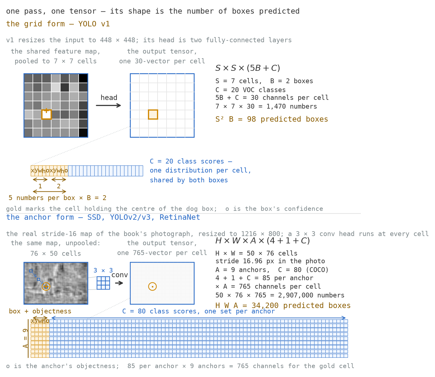
YOLO uses the simplest version of that layout [1]. It divides the image into an \(S \times S\) grid. Each cell predicts \(B\) boxes, each with centre coordinates relative to the cell, width and height relative to the image, and one confidence. The cell also predicts one class distribution over \(C\) classes, shared by all \(B\) of its boxes, so the output is \(S \times S \times (5B + C)\).
At the paper’s PASCAL VOC setting of \(S = 7\), \(B = 2\) and \(C = 20\), the network emits a \(7 \times 7 \times 30\) tensor from a \(448 \times 448\) input: 1,470 numbers describing 98 candidate boxes for the whole image. The RPN of Section 4.4 scores tens of thousands of anchors on the same photograph.
Assignment is by centre. The cell containing an object’s centre is responsible for that object, and within that cell, the box whose current prediction has the highest IoU with the ground truth is the one trained on it. Everything else counts as background.
The loss is a sum of squared errors throughout, with two hand-set constants balancing the terms. \(\lambda_{\text{coord}} = 5\) scales the coordinate terms up, and \(\lambda_{\text{noobj}} = 0.5\) scales down the confidence terms of empty boxes. The lower no-object weight limits the contribution from empty cells; without it, their combined gradient overwhelms the few cells assigned to objects. Width and height are regressed as square roots, so a ten-pixel error on a small box costs more than the same error on a large one.
YOLO reaches 63.4 mAP on VOC 2007 at 45 frames per second; Fast YOLO, with nine convolutional layers instead of twenty-four, reaches 52.7 mAP at 155. Both were timed on a Titan X with no batching [1]. Faster R-CNN with VGG-16 sits at 73.2 mAP and 7 frames per second in the same table, so YOLO runs about 6.4 times faster and scores 9.8 mAP lower.
The YOLO paper shows where YOLO and Fast R-CNN make different errors. Localisation errors make up more of YOLO’s mistakes than all other error types combined, while Fast R-CNN produces background false positives nearly three times as often: 13.6% of its top detections contain no object, against 4.75% of YOLO’s. The paper also reports that YOLO “struggles with small objects that appear in groups, such as flocks of birds”. Its output layout explains why: one cell can report only two boxes and one class distribution. Figure 5.2 demonstrates the limit on our image.
The widget overlays the grid on our image. Each cell holds one slice of the output tensor: \(B\) boxes of four coordinates and a confidence, then a single class distribution for the whole cell. Clicking a cell lays that slice out number by number and draws its boxes on the image. The cell containing the dog’s centre, \((448.5, 493.5)\) in the photograph’s \(1264 \times 848\) pixels, is marked. Under YOLO’s rule it is the only cell responsible for the dog, however much of the animal its neighbours cover.
At \(S = 7\) and \(B = 2\), work out how many candidate boxes exist for the whole photograph, and how many objects the cells along the dog’s back could report between them. Then change \(S\) and \(B\), and compare the tensor shape with the box count. The grid chips run 7, 13 and 19, and then the real \(50 \times 76\) stride-16 map of Figure 5.1. The ground-truth box is the one drawn by hand for this book in Section 4.1.
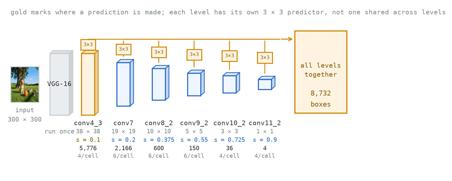
SSD keeps dense prediction but reads six feature maps at different resolutions, each with its own predictor [2]. The paper is explicit that “the convolutional model for predicting detections is different for each feature layer”, so the weights are not shared between levels; a \(3 \times 3\) convolution at one level emits that level’s boxes and nothing else. For the 300-pixel model those are conv4_3 at \(38 \times 38\), conv7 at \(19 \times 19\), then \(10 \times 10\), \(5 \times 5\), \(3 \times 3\), and conv11_2 at \(1 \times 1\). Each level carries default boxes, which are the anchors of Section 4.4 under another name, and the scale of a default box is set by the level it sits on, spread linearly from 0.2 to 0.9 of the image. The paper then overrides the finest level by hand: conv4_3 takes 0.1 on the VOC models and 0.07 on the COCO ones, below the bottom of that range. Figure 5.3 draws the six levels and where each predicts.
figures/verify_numbers.py.
The shapes at a level are the aspect ratios \(\{1, 2, 3, \tfrac12, \tfrac13\}\) plus one extra square box at the intermediate scale \(\sqrt{s_k s_{k+1}}\), six in all. Three levels use all six; conv4_3, conv10_2 and conv11_2 omit the 3 and \(\tfrac13\) ratios and use four. A small object is handled by a level whose stride is fine enough to resolve it, rather than by a small default box on a coarse level. SSD thus uses the multi-resolution maps produced by the network’s downsampling instead of building the image pyramid of Section 1.5 by hand.
Count them:
\[ 38^2 \!\cdot\! 4 + 19^2 \!\cdot\! 6 + 10^2 \!\cdot\! 6 + 5^2 \!\cdot\! 6 + 3^2 \!\cdot\! 4 + 1^2 \!\cdot\! 4 = 5{,}776 + 2{,}166 + 600 + 150 + 36 + 4 = 8{,}732 . \]
That’s 8,732 default boxes per image against YOLO’s 98. Almost all of them are background, and two thirds sit on the finest level, where the cells are smallest and objects are rarest.
SSD therefore uses hard negative mining. It sorts the negatives by their confidence loss, retains at most three of the highest-loss negatives per positive, and excludes the rest from the classification loss. YOLO’s \(\lambda_{\text{noobj}}\) and SSD’s mining reduce the same imbalance, and both do it by down-weighting or discarding most of the negatives.
Table 7 of the SSD paper lists the box counts beside the frame rates on VOC 2007 test [2]. SSD’s rows were timed on a Titan X with cuDNN v4. The Fast YOLO, YOLO (VGG-16) and Faster R-CNN values were copied from Table 1 of the YOLO paper and measured separately, also on a Titan X:
| Method | Input | Boxes | mAP | FPS | Batch |
|---|---|---|---|---|---|
| Faster R-CNN (VGG-16) | ~1000 × 600 | ~6,000 | 73.2 | 7 | 1 |
| Fast YOLO | 448 × 448 | 98 | 52.7 | 155 | 1 |
| YOLO (VGG-16) | 448 × 448 | 98 | 66.4 | 21 | 1 |
| SSD300 | 300 × 300 | 8,732 | 74.3 | 46 | 1 |
| SSD512 | 512 × 512 | 24,564 | 76.8 | 19 | 1 |
| SSD300 | 300 × 300 | 8,732 | 74.3 | 59 | 8 |
| SSD512 | 512 × 512 | 24,564 | 76.8 | 22 | 8 |
Batch size affects reported throughput, so the batch-1 rows give the relevant comparison: SSD300’s 59 frames per second comes from a batch of 8, while Faster R-CNN’s 7 is a batch of 1. Like for like, that’s 46 against 7, a factor of 6.6 rather than 8.
The row marked YOLO (VGG-16) is a third architecture, not the 63.4 mAP model above. The YOLO paper reports a version of the same design on a VGG-16 backbone, which trades most of the speed for 66.4 mAP. SSD300 is both faster and more accurate than that model while scoring 89 times as many boxes. At 46 frames per second SSD300 spends 21.7 ms on its 8,732 boxes, 2.5 µs each, and the VGG-16 YOLO at 21 frames per second spends 47.6 ms on its 98, 486 µs each. These quotients include the whole forward pass; they aren’t the time spent processing one box in isolation.
These figures are only comparable with each other. VOC mAP averages over classes at a single IoU threshold of 0.5, while COCO’s AP (Section 4.1) averages over ten thresholds from 0.50 to 0.95 and gives much lower values for the same detector. Frame rate also depends on the GPU and software used for the measurement. Every remaining result in this chapter uses COCO, and Section 5.4 compares speed on matched hardware.
5.2 Focal loss and RetinaNet
RetinaNet runs its head on FPN levels P3 to P7, at strides 8, 16, 32, 64 and 128, with nine anchors at every location. On an \(800 \times 800\) input those levels hold \(100^2 + 50^2 + 25^2 + 13^2 + 7^2 = 13{,}343\) locations, giving \(120{,}087\) anchors; the paper rounds this to about 100k [3].
A photograph with a dozen objects produces a few dozen positive anchors, since the assignment rule matches every anchor that overlaps a box well enough. The calculation below uses twelve positives as a conservative illustration; its purpose is to show the scale of the imbalance rather than model one image exactly.
Chapter 2 defined cross-entropy as \(-\log p_t\), where \(p_t\) is the probability the model assigned to the true class (Section 2.6). On a well-classified negative that value is small but not zero: an anchor the model is already confident is background, at \(p_t = 0.9\), still costs \(-\log 0.9 = 0.105\).
Multiply that by 100,000 and the background contributes 10,536, while twelve positives at \(p_t = 0.5\) contribute \(12 \times 0.693 = 8.3\). The background outweighs the foreground by 1,267 to 1, leaving the objects with 0.08% of the summed loss. No single easy negative matters much; the problem is their number, because the gradient depends on the sum of all hundred thousand.
Earlier dense detectors reduced the imbalance by down-weighting or selecting negatives. YOLO’s \(\lambda_{\text{noobj}}\) scales the empty cells down, SSD’s hard negative mining keeps three negatives per positive, and online hard example mining (OHEM) builds each minibatch from the highest-loss examples and drops the rest. On a ResNet-101-FPN at 600 pixels, the paper’s best OHEM configuration reaches 32.8 AP, whereas focal loss reaches 36.0.
At \(\gamma = 2\), an example the model already classifies correctly at \(p_t = 0.9\) is multiplied by \((1 - 0.9)^2 = 0.01\), so it contributes a hundredth of its cross-entropy. One at \(p_t = 0.99\) is multiplied by \((1 - 0.99)^2 = 10^{-4}\) and contributes a ten-thousandth. A hard positive still at \(p_t = 0.3\) is multiplied by \(0.7^2 = 0.49\) and changes little. Every example still contributes; the easy ones are simply reduced much further than the hard ones. Figure 5.4 draws the family.
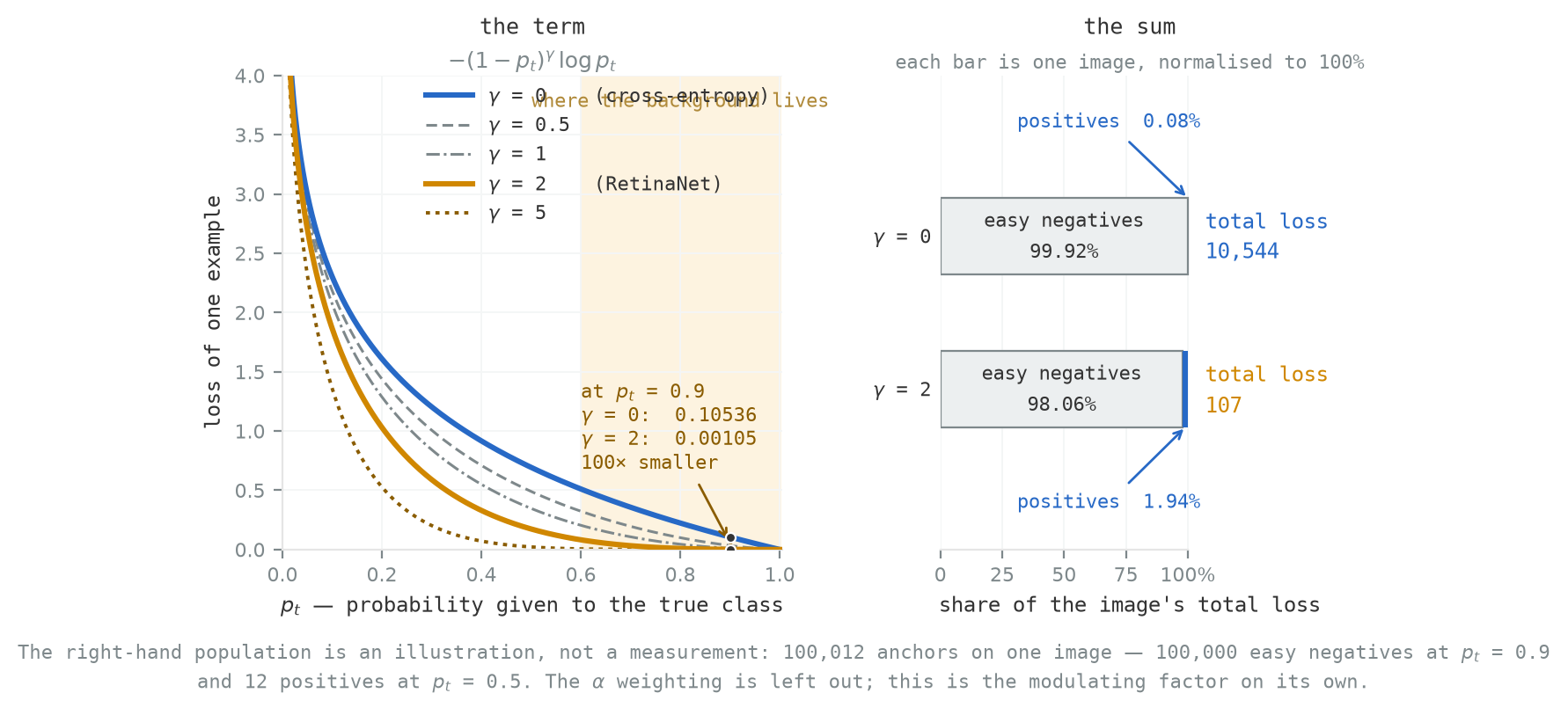
With \(\gamma = 2\) and \(\alpha_t\) held at 1, the calculation isolates the modulating factor: the 100,000 easy negatives now contribute \(100{,}000 \times (1 - 0.9)^2 \times 0.105 = 105.4\) between them. The twelve positives contribute \(12 \times (1 - 0.5)^2 \times 0.693 = 2.08\).
The ratio falls from 1,267 : 1 to 51 : 1, and the foreground’s share of the total rises from 0.08% to 1.9%, a factor of about twenty-five, with no example discarded. Both totals fall at the same time, the background by a factor of a hundred and the foreground by four. The difference between those two factors is what shifts the balance.
The published setting is \(\gamma = 2\) with \(\alpha = 0.25\). Since \(\alpha_t\) is \(\alpha\) on foreground anchors and \(1 - \alpha\) on background, this weights the dozen positives at 0.25 and the hundred thousand negatives at 0.75. Ordinary class balancing would usually do the reverse.
The modulating factor explains the setting: it has already reduced easy examples relative to hard ones, and the hard examples are overwhelmingly positive. A smaller \(\alpha\) offsets some of that shift. Lin et al. report that \(\alpha\) should decrease as \(\gamma\) increases.
On a ResNet-50-FPN at 600 pixels, the best \(\alpha\) falls from 0.75 at \(\gamma = 0\) to 0.25 at \(\gamma = 2\). AP rises from 31.1 to 34.0, then falls to 32.2 at \(\gamma = 5\), but these values use a different backbone and table from the 36.0 quoted against OHEM, so they aren’t directly comparable. Figure 5.5 splits the total between the three groups, with both parameters adjustable.
RetinaNet also changes the classifier’s initial bias and the loss normalisation. The classification layer starts with a bias of \(b = -\log((1 - \pi)/\pi)\) at \(\pi = 0.01\), so at the first step the network predicts foreground with probability about 0.01 rather than 0.5. Without it, a hundred thousand anchors are confidently wrong in the same direction and the first iterations are unstable. Separately, the image’s total loss is normalised by the number of anchors assigned to a ground-truth box, not by the total anchor count. Dividing by 100,000 would make the loss a mean over background.
The widget divides a dense head’s loss among easy negatives, hard negatives and positives, using 100,000 anchors with the \(p_t\) distribution printed on screen plus a dozen positives. The distribution has a plausible illustrative shape; it isn’t a measurement from a trained model. The stacked bar gives each group’s share of the total loss.
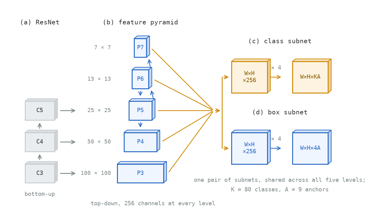
RetinaNet is the detector built to test the loss, and it reuses existing components. A ResNet-FPN backbone (Section 4.5) supplies levels P3 to P7. Nine anchors sit at every location: three aspect ratios \(\{1{:}2, 1{:}1, 2{:}1\}\) times three scale multipliers \(\{2^0, 2^{1/3}, 2^{2/3}\}\), over base areas from \(32^2\) on P3 to \(512^2\) on P7, so the largest square anchor is \(512 \cdot 2^{2/3} = 813\) pixels on a side. An anchor is positive at IoU \(\geq 0.5\) against a ground-truth box and background below 0.4; between the two it is ignored.
Two small subnets read every level, sharing their weights across levels but not with each other. Each is four \(3 \times 3\) convolutions of 256 channels with ReLU, followed by one more \(3 \times 3\) convolution. The classification subnet ends in \(KA\) sigmoid outputs, for \(K\) classes and \(A = 9\) anchors; the box subnet ends in \(4A\) linear outputs, is class-agnostic, and is trained under the smooth \(L_1\) loss of Section 4.3. The training loss is the sum of the two, and there’s no second stage anywhere in the model. Figure 5.6 draws the backbone, the pyramid and the two subnets together.
figures/verify_numbers.py.
RetinaNet with a ResNet-101-FPN backbone at 800 pixels reaches 39.1 AP on COCO test-dev. In the same table, Faster R-CNN with FPN reaches 36.2, the strongest two-stage entry reaches 36.8, and the strongest one-stage entry reaches 33.2; a ResNeXt-101-FPN variant of RetinaNet reaches 40.8 [3]. RetinaNet combines the pyramid of Section 4.5 and the anchors of Section 4.4 with a convolutional head, then changes the training objective to focal loss.
5.3 Anchor-free: FCOS
Anchors give the network reference shapes that it only has to correct, which is an easier learning problem than regressing a box from nothing (Section 4.4). Their scales, ratios and number are selected manually. FCOS removes them and regresses four distances from each feature-map location instead [4]. For a location that maps to pixel \((x, y)\) in the input, the targets are its distances to the four sides of the box containing it:
\[ l^* = x - x_0, \qquad t^* = y - y_0, \qquad r^* = x_1 - x, \qquad b^* = y_1 - y , \]
for a ground-truth box \((x_0, y_0, x_1, y_1)\). All four distances are positive for a location inside the box, and the box is recovered by subtraction as \((x - l,\; y - t,\; x + r,\; y + b)\). FCOS makes one prediction per location instead of nine, which the paper reports as nine times fewer network output variables. Producing a value at every map location is per-pixel prediction in the sense Chapter 6 makes precise.
Assignment is by containment. A location is a positive example for a class if it falls inside a ground-truth box of that class, which makes every interior location positive rather than only those an anchor happens to overlap.
A size rule then selects the pyramid level: a level accepts a location only when \(\max(l^*, t^*, r^*, b^*)\) falls in its range. The boundaries are \(m_2 \ldots m_7 = 0, 64, 128, 256, 512, \infty\): 0–64 on P3, 64–128 on P4, 128–256 on P5, 256–512 on P6, and 512 upwards on P7. A location outside its level’s range is negative even when it lies inside a box. This replaces both the anchor scales and the level-assignment rule of Section 4.5.
The level ranges also separate overlapping boxes of very different sizes, and if a location still falls inside two boxes on the same level, FCOS assigns it to the smaller one.
The FCOS paper measures both effects. With the pyramid in place only 7.14% of positive locations remain ambiguous, against 23.16% without it. Counting the ground-truth boxes that at least one positive location can reach, FCOS’s best possible recall on COCO is 98.40%, against 90.92% for RetinaNet’s official anchor matching. The inside-the-box rule therefore leaves fewer objects without a training signal than RetinaNet’s IoU-based assignment. Figure 5.7 shows both rules on one box.
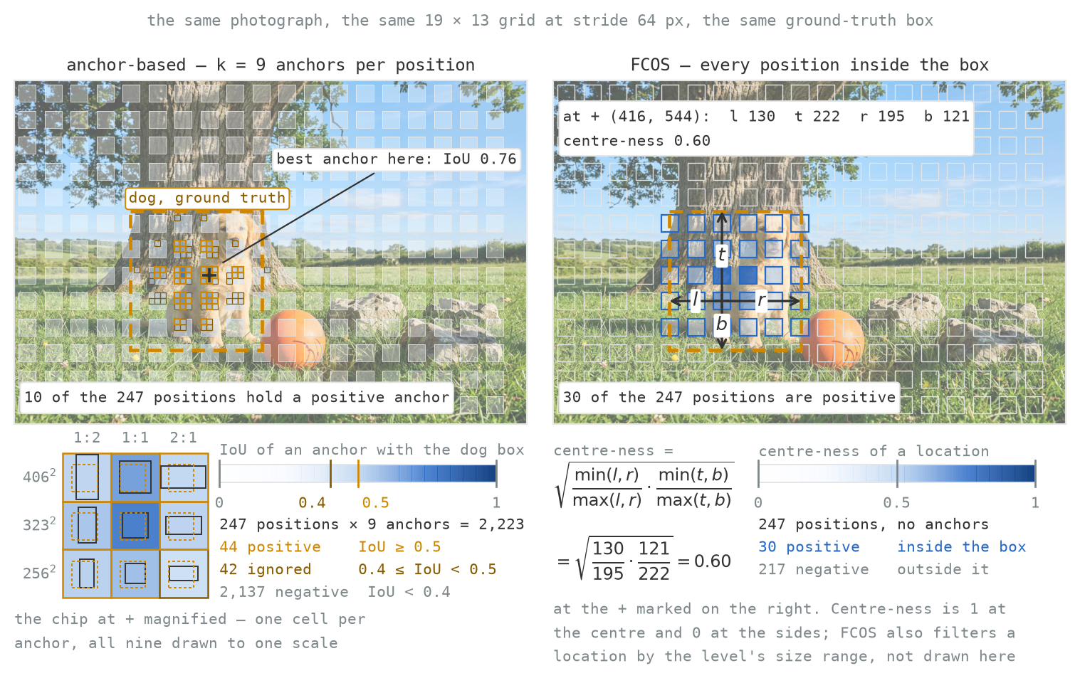
This assignment creates a problem near the box edge, where one target distance is very short and the opposite one very long, so predictions from these locations tend to be inaccurate. The classification branch is independent of the box branch, so a poor box can still receive a high class score and survive thresholding. FCOS therefore predicts how central each location is and includes that value in the ranking.
Figure 5.8 draws the field over a real box and lets you read a location’s four distances off it. The ablation isolates the effect on a ResNet-50-FPN: 33.5 AP without centre-ness and 37.1 with it, on COCO minival, so 3.6 AP for one output channel and one multiplication at test time.
A control row in the same table explains why the extra channel is needed: centre-ness computed from the regressed box, rather than predicted separately, scores 33.5, which is no gain at all. The regressed coordinates contain no independent estimate of their own error; centre-ness has to be predicted separately.
The widget maps centre-ness over the dog’s box, \((286, 322, 611, 665)\), which was drawn by hand for this book. Click any location inside the box to read its four distances, the box those four numbers reconstruct, its centre-ness, and a classification score before and after the multiplication. Pick a location near the muzzle and one near the middle of the body, and compare their scores before looking at their centre-ness. The toggle at the top removes the multiplication and re-counts what clears the score threshold: at the default threshold, 88 of the 440 locations survive with centre-ness, and all 440 without it.
FCOS removes the anchor scales, aspect ratios, number of anchors per location, positive and negative IoU thresholds, and the anchor-to-ground-truth IoU computation used during training. It replaces them with five level ranges and one tie-break rule. The ranges are distances in pixels rather than combinations of reference shapes and overlap thresholds.
RetinaNet is sensitive to its anchor settings: the paper reports a spread of up to 4 COCO AP as they vary. In the reported comparison, removing anchors doesn’t reduce accuracy. FCOS with a ResNet-101-FPN reaches 41.5 AP on COCO test-dev against RetinaNet’s 39.1 on the same backbone, and 43.2 with a ResNeXt-64x4d-101-FPN [4]. NMS remains. Two neighbouring locations inside the same dog can both predict that dog, and the training loss has no term that penalises the duplicate.
5.4 Remaining hand-designed components
RetinaNet’s fixed choices fall into three groups. Anchor assignment: three aspect ratios, three scale multipliers, base areas from \(32^2\) to \(512^2\), and IoU thresholds of 0.5 and 0.4. Loss and training: \(\gamma = 2\), \(\alpha = 0.25\), the bias prior \(\pi = 0.01\), and equal weighting of the classification and box loss terms. Inference: a confidence threshold of 0.05, a cap of 1,000 candidates per pyramid level, and an NMS threshold of 0.5.
FCOS deletes the four anchor-assignment settings and adds five level ranges and a tie-break rule of its own. It keeps the focal loss, and \(\gamma\) and \(\alpha\) with it. These values are manually chosen; several were selected by grid search on a validation set.
NMS differs from the rest of that list. It operates after the network, receives no gradient, and is never trained (Section 4.1), so the model has no way to learn that another location has already claimed an object.
NMS cannot distinguish two overlapping objects of the same class from one object detected twice. Figure 4.7 runs the algorithm on our image, and Figure 4.6 shows the case it cannot resolve: two puppies whose correct boxes overlap at 0.334. A threshold low enough to delete the duplicate also deletes a real animal.
Figure 5.9 plots COCO AP against inference time for the detectors covered so far.
The plot puts COCO AP against inference time per image, one point per published measurement. Colour gives the lineage, one-stage blue and two-stage gold, and the marker gives the timing hardware: filled for an Nvidia M40, hollow for a Titan X.
The Nvidia M40 view holds only measurements taken the same way: the ten RetinaNet configurations in the focal-loss paper’s speed–accuracy table (ResNet-50 and ResNet-101, each at test scales 400, 500, 600, 700 and 800), the Faster R-CNN with FPN result reported alongside them, and Mask R-CNN’s box AP [3], [5]. All use COCO test-dev. The best RetinaNet result in this view is 37.8 rather than the 39.1 quoted above because the 39.1 model used scale jitter and trained for 1.5 times longer.
On COCO test-dev, timed on the same Nvidia M40 in the same paper, RetinaNet with ResNet-101-FPN at 600 pixels reaches 36.0 AP in 122 ms per image, while Faster R-CNN with FPN reaches 36.2 AP in 172 ms [3]. Their reported AP differs by 0.2, and RetinaNet takes 71% as long per image.
Lab 5 produces the same two measurements on your own data. You fine-tune a YOLO on images your group annotated, sweep its confidence and NMS thresholds, and time its throughput against Lab 4’s Faster R-CNN, fine-tuned on the same split and timed on the same machine. The lab then compares two ways of degrading the dataset, halving the training images against corrupting half their labels, and measures which costs more test AP.
These choices arise because a dense detector predicts many candidates at fixed spatial locations and then filters them. Anchor-based detectors add reference shapes at each location and FCOS replaces those shapes with size ranges, but both need assignment rules during training, and both use NMS because neighbouring locations can predict the same object.
A detector that emits a set replaces these local assignment rules with one-to-one matching. It predicts a small fixed number of outputs and matches them against the ground-truth objects using an assignment algorithm inside the loss. There are no anchor shapes or size ranges to choose, and producing two boxes for one object is penalised during training rather than removed afterwards. Chapter 10 builds such a detector.
Object detectors are used in surveillance, where errors can lead to people being misidentified. Gender Shades documents demographic disparities in commercial face-analysis systems [6].
Exercises
- The output tensor. YOLO’s layout at a different setting: \(S = 13\), \(B = 5\), \(C = 80\). Give the output tensor’s shape, the total count of predicted numbers, and the number of candidate boxes. Then explain in one sentence why raising \(B\) from 2 to 5 does not let one cell report five objects of different classes, and say in one more how SSD’s layout differs.
- Counting default boxes. SSD300 predicts from six levels of sizes \(38, 19, 10, 5, 3, 1\), with 4 default boxes per location on the first, fifth and sixth and 6 on the rest. Verify the published total of 8,732. SSD512 adds a seventh level, with sizes \(64, 32, 16, 8, 4, 2, 1\) and box counts \(4, 6, 6, 6, 6, 4, 4\); compute its total and check it against the table above. In each case, what fraction of all boxes lies on the finest level, and what does that imply about which level dominates the classification loss?
- The modulating factor. Compute \((1 - p_t)^\gamma\) and the resulting loss at \(p_t = 0.9\) and \(p_t = 0.1\), for \(\gamma = 0\), \(2\) and \(5\), taking cross-entropy as \(-\log p_t\). Give the ratio of the hard example’s loss to the easy one’s in each case (you should get about 22, 1,770 and 1.3 million). Then state in one sentence what a very large \(\gamma\) risks.
- Where the loss goes. An image produces 100,000 anchors: 20 positives at \(p_t = 0.4\), 99,000 easy negatives at \(p_t = 0.99\), and 980 hard negatives at \(p_t = 0.7\). Compute each group’s share of the total loss under (a) cross-entropy and (b) focal loss with \(\gamma = 2\), \(\alpha = 0.25\). Which group gains the most share, and was it the one you expected? Then say in one sentence what the absolute totals do while those shares are moving.
- FCOS by hand. Our image carries a dog at \((286, 322, 611, 665)\) pixels. For the input location \((400, 500)\): compute \((l^*, t^*, r^*, b^*)\), reconstruct the box from those four numbers, compute the centre-ness, and say which pyramid level takes that location as a positive under FCOS’s ranges. Repeat for \((320, 360)\), which lands on a different level. If the classifier gives both locations a score of 0.8, what score does each carry into NMS, and which survives?
- Under a budget. A detector must run at 10 frames per second on one GPU with no batching, or 100 ms per image. Using Figure 5.9: which configurations are candidates, which is the most accurate of them, and how much AP does the budget cost against the most accurate model on the plot? What does the hover readout tell you to check before comparing two points? Then say what you would change if the budget were 200 ms, and name two changes to the problem you would try before changing the model.
- What NMS cannot fix. In one image two people stand shoulder to shoulder and their ground-truth boxes overlap at IoU 0.78; the detector proposes both, correctly. In another, one person stands alone and the detector proposes two boxes for them, overlapping at IoU 0.55. Work out the range of class-wise NMS thresholds that keeps the pair, and the range that removes the duplicate, and show that they do not meet. Then say what a detector would have to emit for the problem to disappear, and what its training loss would have to penalise for the detector to learn that behaviour.
Lab 5
Lab 5: annotate a small dataset (CVAT/Roboflow), and measure how far two annotators disagree; fine-tune a pretrained YOLO on it; sweep confidence and NMS thresholds; profile speed against Lab 4’s Faster R-CNN; and weigh more data against better labels.

Further reading
- Redmon et al. [1] — YOLO; section 4.2’s error analysis splits each detector’s mistakes into localisation and background errors, which is where the mAP gap with Fast R-CNN is accounted for.
- Liu et al. [2] — SSD; Table 7 gives the box counts, frame rates and batch sizes together, and Table 3 removes prediction layers one at a time to isolate what multi-scale prediction contributes.
- Lin et al. [3] — focal loss; the cumulative loss distributions show how much of the total comes from easy negatives, and the \(\gamma\)–\(\alpha\) sweep is the ablation the setting comes from.
- Tian et al. [4] — FCOS; the ablations remove one hand-set constant at a time and report the cost in AP, and the centre-ness table includes a control row that computes centre-ness from the regressed box instead of predicting it.
- Lin et al. [7] — FPN; every detector in this chapter uses one as its backbone.
- Everingham et al. [8] and Lin et al. [9] — the VOC and COCO metric definitions, which show why mAP at a single IoU threshold and AP averaged over 0.50–0.95 cannot be compared.