1  Images, Filters, and Hand-Crafted Vision

NoteLearning objectives

• Explain how a scene becomes an array: pinhole projection, pixels and subpixels, sampling, quantisation, aliasing, and colour spaces
• Manipulate tone with point operations: brightness, contrast, gamma, stretches, and histogram equalisation
• Implement 2D convolution and understand it as the primitive of the whole course
• Detect edges (Sobel, Canny) and reason about scale via image pyramids
• Measure how classical features degrade under noise
• Describe texture with Gabor filters, the MR8 filter bank, and textons
• Build a Bag-of-Visual-Words classifier and recognise the codebook recipe

Skills ladder. Colab fluency and notebook hygiene; CPU vs GPU runtimes.

An image is an array of numbers. A filter is a much smaller array of numbers. Slide the second over the first, multiplying and summing at each position, and structure appears: edges, scales, textures. Summarise the responses, cluster the summaries into a vocabulary, count the vocabulary, and you have a classifier. That pipeline, filter, describe, cluster, count, was the state of the art in computer vision for roughly a decade, and every stage of it was designed by hand.

This chapter builds the whole pipeline, start to finish. The rest of the book replaces its stages one by one with learned versions, which is why the course spends only this week on the classical material. Most of it returns later: the convolution defined here is the primitive of every network in the book, and where a later chapter reuses something from this one, the text says so at both ends.

One deferral, so you know where you stand. Camera geometry, meaning where a camera sits in three-dimensional space and how to reason backwards from an image to it, waits for Chapter 16. This chapter needs only enough of the camera to know what an image is.

1.1 Image formation

1.1.1 The pinhole camera

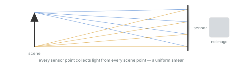
Light leaves every point of a scene in every direction. Hold a bare sensor up to it and no image forms: each point of the sensor receives light from every point of the scene, all summed together (Figure 1.1). An image requires correspondence: each sensor point receiving light from one scene point only. Blur and noise are both correspondence partly lost.

Figure 1.1: A bare sensor. Light from every scene point reaches every sensor point, so no image forms and the sensor records a uniform smear.

The pinhole can provide correspondence. Place an opaque barrier in front of the sensor and make a small hole. Of all the rays leaving a scene point, only the one aimed at the hole gets through, so each sensor position receives light from a single scene point, and an image forms. Rays from high scene points travel down through the hole and rays from low points travel up, so the image is inverted (Figure 1.2). This is the camera obscura, known for over a thousand years; what was missing until the 1820s was a way to make the image permanent.

Your eye is a camera obscura too: the image on your retina is upside-down. The flipping is done in the brain.

Figure 1.2: The pinhole camera. A barrier with a small hole, the aperture, admits one ray per scene point; rays cross at the optical centre, so a sharp, inverted image forms on the sensor at focal length \(f\). The dashed line through the optical centre, perpendicular to the sensor, is the optical axis. The small square beside the sensor shows what it records.

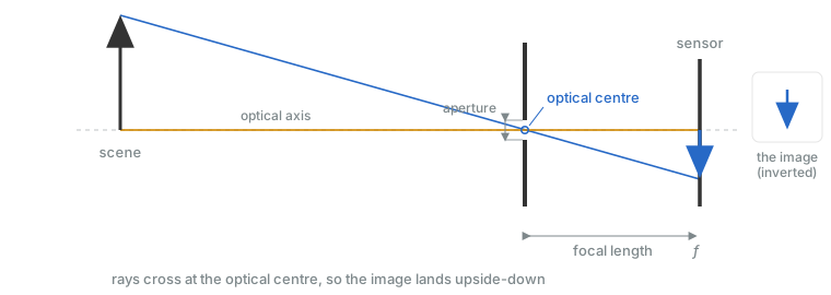
The hole is called the aperture. The idealised point at the centre of the aperture is the optical centre. The literature also calls it the camera centre or the centre of projection, and all three terms are used interchangeably. The optical axis is the line that passes through the optical centre and is perpendicular to the sensor. The sensor itself is positioned behind the aperture at a distance equal to the focal length \(f\).

The rays form similar triangles on either side of the optical centre. In Figure 1.3, the scene point, its foot on the optical axis, and the optical centre form a triangle with height \(h\) and base \(Z\); past the aperture, the same ray forms a second triangle with height \(h'\) and base \(f\). The triangles are similar, so

\[ \frac{h}{Z} = \tan(\theta) = \frac{h'}{f} \Rightarrow h' = \frac{h\,f}{Z}. \]

Figure 1.3: The similar triangles behind \(h' = hf/Z\). One ray runs from the scene point through the optical centre to the image point. On the scene side it spans a triangle of height \(h\) and base \(Z\); on the sensor side, height \(h'\) and base \(f\). The angle \(\theta\) is the same on both sides of the optical centre, so \(h/Z = \tan\theta = h'/f\).

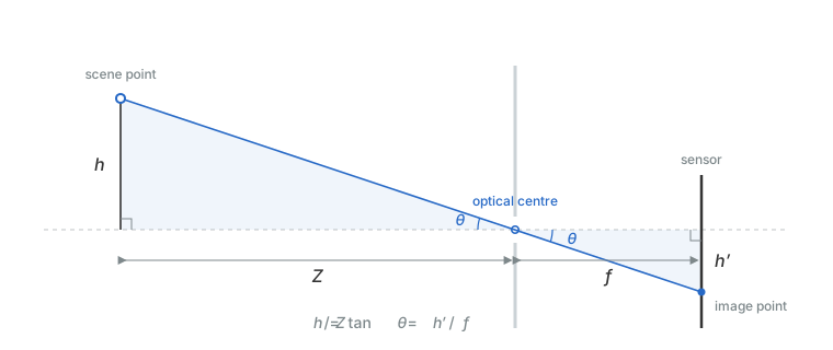
Double \(f\) and the image doubles: zoom. Double \(Z\) and it halves: perspective. In the widget below, the trace buttons draw both triangles with live numbers.

The same triangle also fixes how much of the scene fits on the sensor. A sensor of extent \(h_s\) has its edge \(h_s/2\) from the optical axis, so the ray landing there leaves the optical centre at an angle whose tangent is \(h_s/2f\). Both edges together give the field of view:

\[ \text{FOV} = 2\arctan\frac{h_s}{2f}. \]

The sensor’s size is fixed by the hardware, so \(f\) alone decides it. On a 40 mm sensor, a 20 mm lens takes in 90°, a 50 mm lens 44°, and a 120 mm lens only 19°: a long lens magnifies by seeing less. Everything outside that wedge misses the sensor entirely. The field of view toggle in the widget below draws the two edge rays, running them backwards from the sensor edges into the scene.

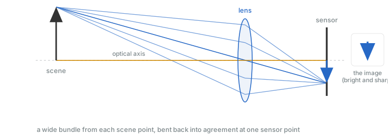
An ideal pinhole passes one ray per scene point: sharp, but almost no light. Widening the hole admits a bundle per point, which lands as a disc about the size of the aperture — brighter and blurrier, and in the limit back to Figure 1.1. Shrinking has a floor too: below roughly 0.3 mm, diffraction blurs the image again. A lens escapes the compromise by gathering a wide bundle from each scene point and bending it back to a single sensor point (Figure 1.4), giving the brightness of a wide aperture with the sharpness of a pinhole. It only works for scene points at the right distance, though; focus and depth of field are the lens’s problems, and we defer them.

Figure 1.4: The lens’s escape. The barrier admitted one ray per scene point and threw the rest away; a lens accepts the whole bundle and bends it back into agreement at a single sensor point, giving the light of a wide aperture with the sharpness of a pinhole. The agreement only holds for scene points at the right distance.

From here on we take the projected image as given. The projection is continuous; making it discrete is the sensor’s job.

Interactive: the pinhole playground

A tree, a dog, a barrier, a sensor. Zoom with \(f\), walk the dog away with \(Z\), open the aperture and watch correspondence dissolve. Five experiments to run:

• The ideal pinhole — one ray per scene point, straight through the optical centre: Figure 1.3, live. Press trace: tree top, read \(h\), \(Z\), and \(f\) off the triangles, and check \(h' = hf/Z\) by hand. Then nudge the aperture off zero — what did the idealisation hide?
• The smallest real hole — a real 0.1 mm hole, and the image is nearly black. A hole admits light in proportion to its area, and area goes as diameter squared: how many times more light does the 10 mm hole collect than this one? This is why real pinhole photographs need exposures of seconds to minutes — and why every practical camera eventually reaches for a lens.
• Bright and blurry — each scene point now sends a bundle of rays, not one. Follow the tree’s bundle and the dog’s bundle to the sensor: where do they overlap? This is Figure 1.1 in the making — what would it take to get all the way there?
• Telephoto — walk the dog closer with the \(Z\) slider. Both grow, but the dog grows faster. Why? (\(h' = hf/Z\) — but whose \(Z\)?) Keep going: at what distance does the dog’s ear ray miss the sensor entirely?
• Field of view — before touching anything: the image can only contain so much of the scene. Which two rays mark that boundary? Where must they pass through, and where must they end? Decide, then switch on field of view to check. Now double \(f\) and predict the new angle from \(2\arctan(h_s/2f)\) before reading it off the wedge.

1.1.2 From scene to pixels

The sensor is a grid of tiny light buckets called photosites. While the shutter is open, each one collects the light that falls on it and reports a single number — more light, a bigger number. The continuous image becomes a table of numbers, one per photosite, in rows and columns.

Each of those numbers is a pixel, short for picture element. Note what that does and does not mean. A photosite must have area, or it would catch no light at all; but what it passes on is one value at one grid position, and that is all the rest of the pipeline ever sees. So a pixel is a sample, a location and a value, not a small square of colour. The squares you see when you zoom into an image are how software chooses to draw samples; they are not what the sensor measured.

On real hardware, though, a pixel is also a physical thing, and at both ends of the pipeline it subdivides further (Figure 1.5). Photosites count light whatever its wavelength, so they cannot tell colours apart, and the sensor lays a mosaic of colour filters over them. Almost always this is the Bayer mosaic: a repeating 2×2 tile of one red, one blue, and two green filters. Each photosite therefore measures one channel, and the other two are interpolated from its neighbours, a step called demosaicing. Two-thirds of the colour numbers in a “raw” photo are estimates, which makes demosaicing the first algorithm to run on almost any photograph. Displays play the same trick in reverse: each screen pixel is built from red, green, and blue subpixels, and “white” is small lights too close together for your eye to separate. Manufacturers arrange them differently: plain stripes; diamond lattices carrying half as many red and blue subpixels as green, so neighbouring pixels draw on the same ones; quads with a white subpixel added for brightness. That disagreement is why a photograph of one screen displayed on another can moiré, and why text rendered for one subpixel order can fringe with colour on a panel built to another.

Figure 1.5: Subpixels at both ends of the pipeline. (a) The sensor’s Bayer mosaic: each photosite sits under a single colour filter, in repeating 2×2 tiles of one red, two green, one blue; demosaicing interpolates each site’s two missing channels. (b) Displays subdivide too, but manufacturers do not agree on how: a plain RGB stripe; PenTile RGBG, which gives every pixel a green subpixel but only every second one a red or a blue; or a four-subpixel layout that adds white for brightness.

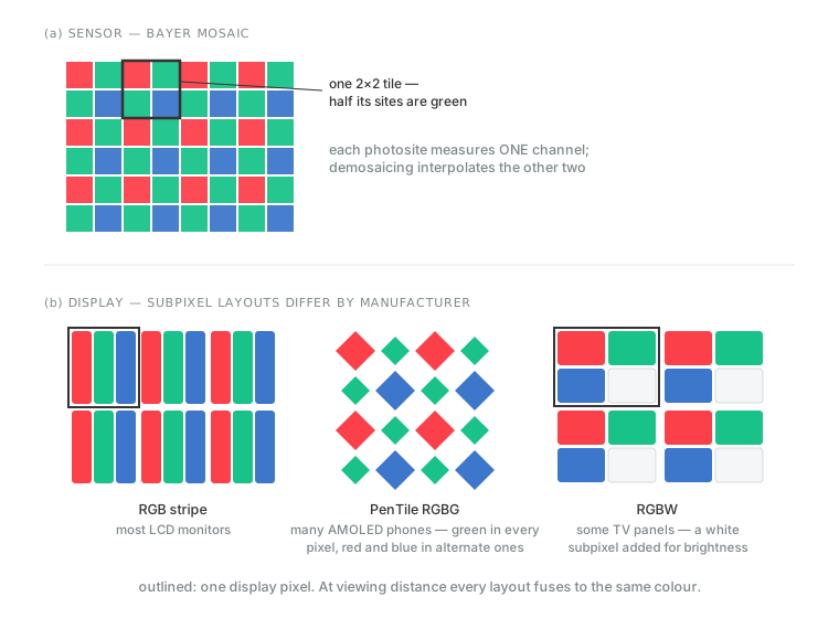
Look at the two panels of Figure 1.5 together and the PenTile lattice should seem familiar: green on half the sites, red and blue on a quarter each, is exactly the Bayer mosaic drawn above it. Sensor and screen arrived at the same arrangement independently, for the same reason: the eye draws most of its detail from green, so that is the channel neither end samples sparsely.

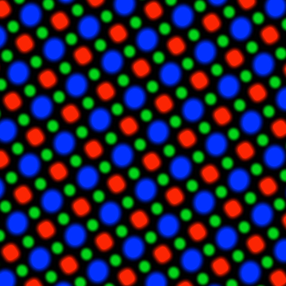
Figure 1.6 shows a real one, reconstructed from a Galaxy S8 panel. The schematic above squares everything off for clarity; on the actual display the lattice is rotated, the green subpixels are noticeably smaller than the red and blue ones, and every subpixel is separated by black. The counting is unchanged: a green for every pixel, a red or a blue for every second one.

Figure 1.6: The diamond PenTile matrix of a Galaxy S8 OLED display: small green subpixels at every pixel position, with larger red and blue diamonds alternating between them. Reconstruction by Louis PL, CC BY-SA 4.0, via Wikimedia Commons.

The triads are worth seeing for real. The Slow Mo Guys film screens up close and in slow motion — watch white dissolve into red, green, and blue:

In code, all of this arrives as an array: height × width for grayscale, height × width × 3 for colour, indexed I[row, column] — row first, and row 0 at the top. The values are either 8-bit integers in \([0, 255]\) or floats in \([0, 1]\). Keep track of which you are holding — mixing them up is a common source of bugs.

WarningThe first NumPy bug you will meet

uint8 arithmetic overflows silently: np.uint8(200) + np.uint8(100) is 44, not 300, and a brightened image full of wrapped-around dark speckles is the classic symptom. Convert to float before doing arithmetic, and only convert back (with clipping) for display. Lab 1 makes you hit this bug on purpose.

1.1.3 Sampling, quantisation, and aliasing

Digitisation makes two independent choices: how many samples to take, and how many values each sample may hold. The first is resolution, the size of the grid. The second is bit depth: a \(b\)-bit image rounds each sample to one of \(2^b\) levels, and the standard 8 bits gives 256 of them.

Figure 1.7 pushes each choice until it breaks, in both directions. Lowering resolution removes detail: the thinnest bars vanish first, then the sun’s soft edge turns to steps. Lowering bit depth breaks smooth variation instead: the gradient splits into flat terraces, called banding or posterisation. The two failures look different because the choices are different: one starves the image of positions, the other of values.

Figure 1.7: One test image, pushed along both axes of digitisation. Top row: shrinking resolution at full bit depth, where fine structure merges and disappears (look at the striped band in the middle panel: it does something stranger than disappear, which is the next figure’s subject). Bottom row: shrinking bit depth at full resolution, where smooth regions terrace into bands. Switch the widget to edit the values to move between these settings yourself.

Losing detail is the failure you expect. Aliasing is the one you do not: sample a pattern too coarsely and it does not fade out. It reappears as a different, coarser pattern that was never in the scene. Figure 1.8 demonstrates it. The zone plate’s rings tighten towards the edge; keeping only every eighth pixel produces broad new rings that exist nowhere in the original. The everyday version is moiré: a striped shirt on television, a distant brick wall in a photo. The limit is Nyquist’s. A pattern survives sampling only if you take more than two samples per cycle of it. Finer patterns are not simply lost; they are folded down to a lower frequency, which is why what comes back looks coarser than what went in.

ImportantThe sampling theorem

Nyquist–Shannon. If a signal \(x(t)\) contains no frequency above \(B\), it is completely determined by its samples taken at any rate \(f_s > 2B\), and is recovered exactly by

\[ x(t) \;=\; \sum_{n=-\infty}^{\infty} x\!\left(\tfrac{n}{f_s}\right)\, \operatorname{sinc}\!\big(f_s t - n\big). \]

Half the sampling rate, \(f_s/2\), is the Nyquist frequency, the highest frequency those samples can represent. Content above it is not discarded. It is folded back below \(f_s/2\) and added to whatever was already there, so the false pattern and the true one become the same numbers: no later processing can separate them. That is the whole reason the fix has to come before sampling, not after.

Images obey the same statement in each spatial dimension, with \(B\) in cycles per pixel: either sample more than twice as finely as the finest detail present, or blur until that is true.

Figure 1.8: Aliasing on a zone plate. Left: the original, where ring frequency increases with radius. Middle: keeping only every eighth pixel invents broad false rings. Right: blurring away the finest rings before subsampling loses detail honestly, inventing nothing.

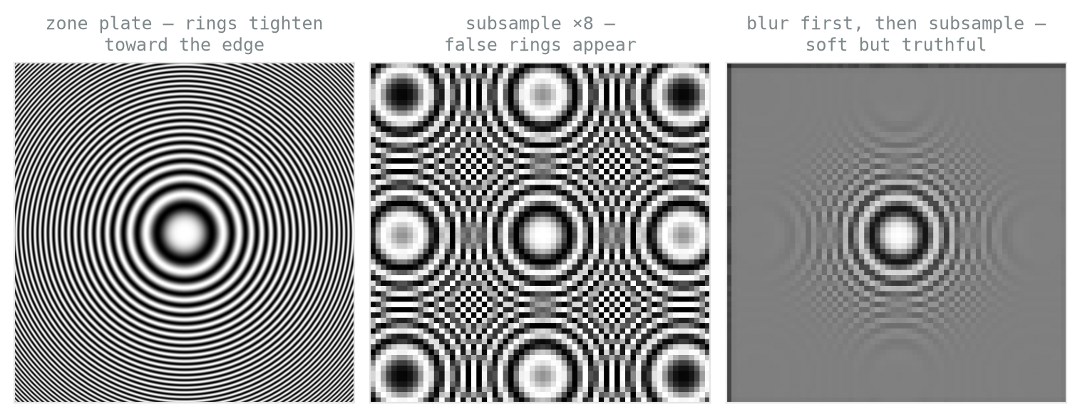
The fix is not more samples. It is to remove, before sampling, the detail the samples cannot carry: blur first, then subsample. The right panel is softer than the original, but every structure in it was present in the scene. Cameras apply the same fix optically, mounting a slight blur filter in front of the sensor.

Interactive: the digitisation playground

Both axes on one image. Push resolution down without the blur and watch the grass alias; toggle the blur on and watch it heal; push bit depth down and watch the sky band. The raw-size readout explains, in passing, why images get compressed.

1.1.4 Colour and colour spaces

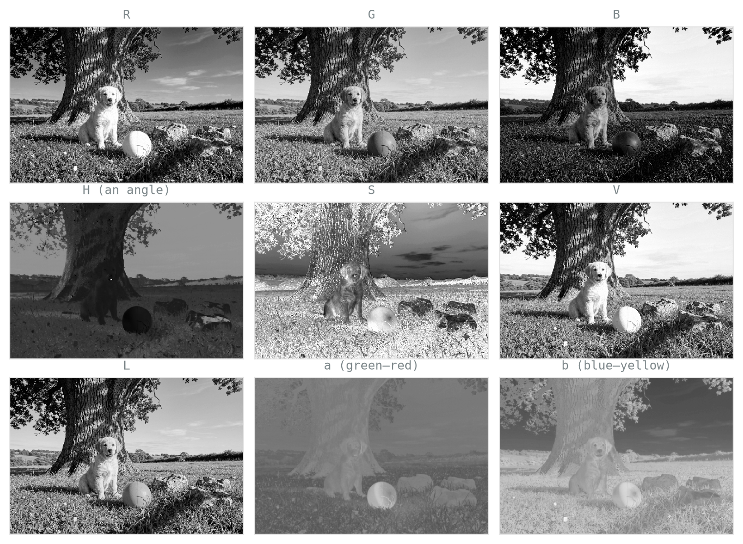
A colour pixel is three numbers, coordinates in the RGB cube. RGB is the native space of the hardware at both ends (the Bayer mosaic measures it, the display triads emit it), but it is an awkward space to reason in, because brightness and colour are entangled across all three coordinates. Move the dog from sun into shade and its R, G, and B all drop together; every “orange” in the scene is a different point, spread along the brightness direction. Figure 1.10, top row, shows the problem: the three channels are nearly the same image three times.

Those three numbers can be re-coordinatised, and Figure 1.9 shows the shapes the common choices take.

Figure 1.9: Five colour spaces, five geometries, the same colours throughout; what changes is which question becomes a single axis. RGB is the additive cube the hardware works in. HSV re-coordinatises it in polar form, so hue is an angle. CMYK is subtractive: inks remove light from white paper, and because three inks together give a muddy brown rather than a true black, printing adds a fourth. L*a*b* and YCbCr both put brightness on the vertical axis. Neither holds a cube of displayable colour: YCbCr is a linear map of RGB, so the cube arrives sheared, while Lab is non-linear and the same colours become a lumpy solid, pinched to black at the bottom and white at the top. Click any of the four solids to open it: drag to rotate, scroll to zoom, and click the surface to read one colour’s coordinates in all four systems.

Converting to grayscale is a weighted sum, \(Y = 0.299R + 0.587G + 0.114B\). The weights are unequal because the eye’s sensitivity peaks in green, the same fact that puts two green sites in every Bayer tile. (Note the form: a dot product between a fixed weight vector and each pixel. Fixed, for now.)

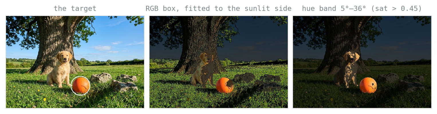
Other spaces re-coordinatise the cube so that useful things become single axes. HSV separates hue (an angle around the colour wheel), saturation, and value: in Figure 1.10, middle row, the ball, a different value in each of R, G, and B, becomes one flat region of the H channel. That makes hue the right axis to threshold on, and Figure 1.11 shows the difference. An RGB box fitted to the sunlit side of the ball loses the shaded side and sprays false positives across the grass, while a single band of hue keeps the whole ball, shadow included. It also claims much of the dog, since in hue terms golden fur is desaturated orange. And hue has a failure mode of its own: it is an angle computed from small channel differences, so on nearly-grey pixels such as the rocks and the clouds it is noise, and it wraps around at red. Threshold saturation alongside it, and do not expect colour alone to finish the job.

YCbCr and Lab split brightness from colour instead. One axis carries brightness, called luma and written Y in YCbCr, lightness and written L* in Lab. The two remaining axes carry chroma, the colour with the brightness removed. YCbCr’s chroma pair are colour differences: Cb measures how far the blue channel sits above the luma, Cr how far the red channel does. JPEG keeps Y at full resolution and stores Cb and Cr at half, because the eye is far sharper about brightness than about colour; in Figure 1.10, bottom row, the two chroma channels visibly carry less spatial detail. Lab instead spaces its axes so that equal distances are roughly equal perceived differences, which is what you want when “how different are these two colours?” is the actual question.

Most of this chapter now proceeds in grayscale: filters, edges, and textures are about structure, and structure lives in brightness.

Figure 1.10: The scene in three colour spaces, one channel per panel. Top: R, G, B, where brightness leaks into all three, so they look like three copies of the same photograph. Middle: H, S, V, where the ball collapses to one flat value in H. Bottom: Lab, where L carries the detail and the a and b chroma channels are smooth and coarse.

Figure 1.11: Segmenting the ball. Left: the target, ringed. Middle: an RGB box fitted to the sunlit side of the ball (mean ± 2.5σ per channel) loses the shaded portion and admits stray grass, rock, and dog pixels. Right: one hue band, 5°–36° with a saturation floor, keeps the ball through the shadow, and claims much of the dog too.

Interactive: segment the ball

Now do better. The sliders control the hue band and the saturation floor; the toggle shows the RGB box you are trying to beat. Target: ball above 95%, dog below 5%. When you get there, work out which slider did the real work.

1.2 Point operations

The simplest thing you can do to an image is transform each pixel on its own: \(I'(x,y) = f(I(x,y))\). These are point operations: the output at a position depends only on the input at that position, through a single function \(f\) applied everywhere. They can move tone around but cannot know where anything is.

1.2.1 Brightness, contrast, and gamma

Brightness and contrast are properties of an image. Brightness is where the values sit overall: the mean intensity, \(\mu\). Contrast is how spread out they are: the standard deviation of the intensities, \(\sigma\), called RMS contrast, or more loosely the range the values span. The two are independent statistics of the histogram, and Figure 1.12 puts one scene in all four corners.

Figure 1.12: One scene, four corners of (brightness, contrast). The histograms below each panel carry the two numbers directly: \(\mu\) is where the mass sits (blue line), \(\sigma\) is how wide it spreads. Left column: high contrast, where at both exposures the histogram piles up against an end of the range, the clipping the next paragraphs return to. Right column: low contrast, the same scene compressed into a narrow band, washed out when bright and murky when dark.

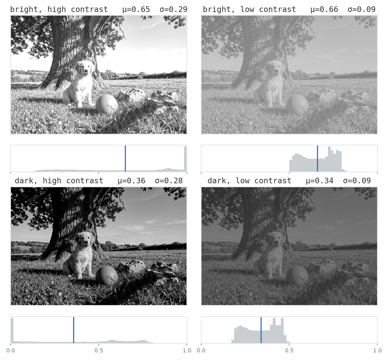
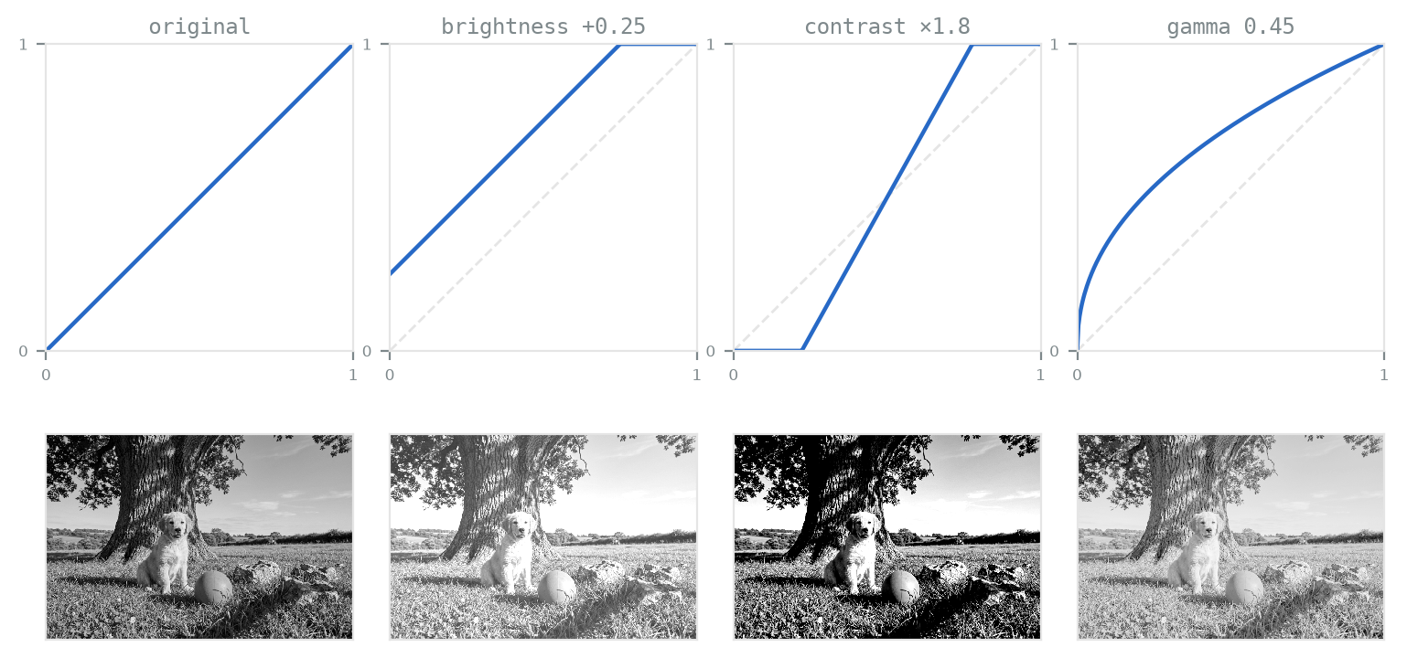
The adjustments named after them, the brightness and contrast sliders of any photo editor, are the point operations that move one statistic at a time. The brightness adjustment is addition, \(f(v) = v + b\): every value moves by \(b\), so \(\mu\) moves by \(b\) and the histogram slides along unchanged in shape, leaving \(\sigma\) where it was. The contrast adjustment is multiplication about the midpoint, \(f(v) = \alpha(v - 0.5) + 0.5\): every deviation from mid-grey is scaled by \(\alpha\), so \(\sigma\) is multiplied by \(\alpha\) (and so is the mean’s own distance from mid-grey). Because a point operation is just a function on \([0,1]\), you can read each from its graph, the transfer curve, input along the bottom and output up the side, in Figure 1.13: addition shifts the line up; multiplication steepens it about the midpoint.

Both of those tidy statements hold only until values reach the ends of the range. Whatever lands past white or black clips, and clipping is the thing to watch: distinct inputs have become the same output, the histogram piles up at 0 or 1, and no later operation can take that back.

The brightness and contrast adjustments are both straight lines, and both clip. Gamma is the standard curved adjustment: \(f(v) = v^{\gamma}\) on \([0,1]\). Its endpoints are pinned, since \(0^{\gamma} = 0\) and \(1^{\gamma} = 1\), so black stays black and white stays white while everything between moves: \(\gamma < 1\) lifts mid-tones (\(0.5^{1/2.2} \approx 0.73\)), \(\gamma > 1\) lowers them (\(0.5^{2.2} \approx 0.22\)). Where brightness and contrast push tones off the ends of the range, gamma redistributes them inside it, so it is the one tone control here that cannot clip.

Gamma also has a second job, built into the data before you ever load it. The eye tells shadow steps apart far better than highlight steps, so spending 256 levels evenly on physical light wastes codes where no one can see them. Stored images therefore apply roughly \(v^{1/2.2}\) before quantising, brightening the encoding so that more of the 256 levels land in the dark tones, and the display raises the values back to the power \({\approx}2.2\) to undo it. This convention is sRGB, the default encoding of essentially every JPEG and PNG you will touch. The consequence: the numbers in your array are not proportional to physical light, so averaging them, which is what blurring does, is subtly wrong. Averaging light that a camera would have averaged means working in linear values. There are two ways to get them. Undo the encoding in software, raising to the power 2.2, filtering, then re-encoding. Or start from the camera’s RAW file, the Bayer-mosaic sensor counts of Section 1.1.2 before demosaicing, white balance, and this encoding ever happen. RAW counts are linear in captured light from the start, and at 12–14 bits they keep precision in the shadows that the 256 encoded levels no longer have; pipelines with physical stakes, such as HDR merging and astronomy, begin there. Almost nobody in everyday vision does either. Standard practice across computer vision, and every lab in this course, is to filter the values exactly as imread hands them over. For the tasks in this book the difference is negligible; where it does show is in rendering and photo compositing, where blurring encoded values visibly darkens the seam between bright colours.

Figure 1.13: Three point operations, each with its transfer curve above its result. The dashed diagonal is the identity. Brightness shifts the curve and clips at white; contrast steepens it about the midpoint and clips at both ends; gamma bends it, brightening mid-tones while pinning black and white.

1.2.2 Histograms, stretches, and equalisation

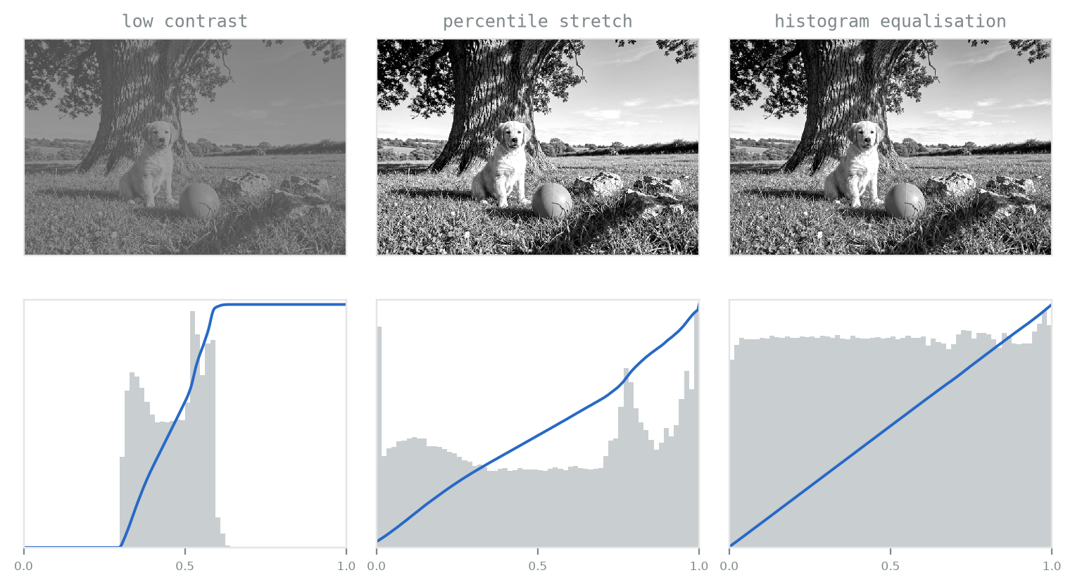
The histogram counts how many pixels hold each value. It is the image’s tonal summary with the geometry thrown away, and exposure problems are legible in it at a glance: a pile-up at zero is crushed shadow, a spike at one is blown highlight, and a narrow hump in the middle (Figure 1.14, left) is a low-contrast image using only a fraction of its range.

The direct fix is a contrast stretch: map the occupied range back to \([0,1]\) with one linear ramp. Use percentiles (say the 2nd and 98th) rather than the true min and max, or a single stray pixel sets the whole mapping. Histogram equalisation goes further: use the image’s own cumulative distribution as the transfer curve, \(f(v) = \mathrm{CDF}(v)\), the fraction of the image’s \(N = HW\) pixels whose value is at most \(v\). Values in crowded regions of the histogram, where the CDF is steep, get spread apart; values in empty regions get pushed together; the result uses essentially the full range with a roughly flat histogram. It shines on fog, underexposure, and X-rays.

Figure 1.14: A low-contrast image repaired two ways. Below each image: its histogram (grey) and cumulative distribution (blue). The stretch spreads the occupied range linearly; equalisation uses the CDF itself as the transfer curve, yielding a roughly flat histogram and a straight CDF.

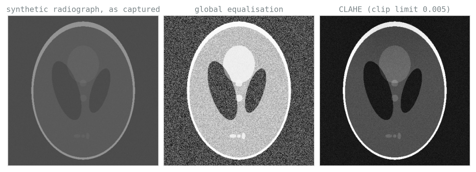
Equalisation also lies. The CDF is steep wherever pixels are crowded, and it cannot tell whether they are crowded because of signal or because of noise. A nearly uniform region is a spike in the histogram either way, and equalisation stretches it regardless. Figure 1.15 runs the failure at full size on a synthetic radiograph (the Shepp–Logan phantom, rendered at low contrast with mild sensor noise). Equalisation makes the anatomy visible and fills the uniform tissue with mottled texture that is not anatomy at all: noise amplified about tenfold into structure that a reader of the image could mistake for something real. Section 1.6 gives us the vocabulary to say this precisely; for an image read for diagnosis, inventing structure is a worse failure than lacking contrast.

The practical repair is CLAHE, contrast-limited adaptive histogram equalisation, and both halves of the name fix one failure. Adaptive: the image is divided into tiles (Figure 1.15 uses a grid of roughly \(4 \times 4\)), each tile gets its own mapping, and every pixel blends the mappings of its four surrounding tiles, so a dark corner and a bright sky are each equalised on their own terms with no visible seams. Contrast-limited: before each tile’s CDF is computed, every histogram bin is clipped at a ceiling and the excess redistributed across all bins. Since the mapping’s slope is the histogram’s height, the ceiling is a direct cap on local contrast gain, and flat noisy regions, the exact places global equalisation goes wrong, hit the cap first. One number, the clip limit, sets how much amplification you will accept.

Figure 1.15: Global equalisation inventing structure. Left: a synthetic radiograph, the Shepp–Logan phantom at low contrast with mild noise; the uniform tissue really is uniform. Middle: global equalisation reveals the anatomy but fills tissue and background with mottled texture that does not exist, amplifying the noise over truly flat regions from σ ≈ 0.01 to σ ≈ 0.10. Right: CLAHE with a clip limit of 0.005 shows the same anatomy while capping the amplification at about a third of that.

Interactive: CLAHE, tile by tile

The widget divides the radiograph of Figure 1.15 into a \(4 \times 3\) grid of tiles, each with its own transfer curve, and adds a draggable probe. The probe’s input value crosses all four surrounding curves at once, giving four different answers, and the rectangle diagram shows how closeness turns into the weights that blend them. Where does the blend matter most? Park the probe on a tile boundary, then switch to nearest tile only and see what the image loses without it. Then lower the clip limit and watch the gold mass in the tile’s histogram, which is the contrast the ceiling has removed.

Interactive: the point-op playground

Every operation of this section on one image. The sliders compose brightness, contrast, and gamma into a single transfer curve, drawn live beside the histogram, with \(\mu\) and \(\sigma\) read out beneath it. Check the definitions above against it: brightness moves only \(\mu\), contrast scales \(\sigma\), until clipping breaks both statements. Two more things to try. Push contrast until the histogram piles up at the ends, which is clipping, and no later slider brings it back. Then switch on equalisation, find the invented texture in the sky, and lower CLAHE’s clip limit until it disappears, watching the curve panel change from one global curve to a bundle of local ones.

1.3 Filtering and convolution

A filter looks at a neighbourhood. In place of \(f(I(x,y))\) we compute each output pixel from a window of input pixels, combining them with a small grid of weights called a kernel. This one operation is the primitive of the entire course: everything from edge detection to the networks of Chapter 2 is built from it.

1.3.1 Correlation, convolution, and the flip

The natural version of the filtering operation is cross-correlation: centre the kernel \(K\) on a pixel, multiply each weight by the pixel underneath it, and sum,

\[ (I \otimes K)(x, y) = \sum_{i}\sum_{j} K(i, j)\, I(x + i,\; y + j). \]

Convolution is the same thing with the kernel flipped through its centre, \(I * K\), using \(I(x - i, y - j)\) instead.

Why does the flip exist at all? With it, convolution is associative: \((I * K_1) * K_2 = I * (K_1 * K_2)\). That property does real work later in this chapter; beyond it, the flip can be ignored.

\[ (I * K)(x, y) = \sum_{i}\sum_{j} K(i, j)\, I(x - i,\; y - j). \]

For the symmetric kernels that dominate this chapter the flip changes nothing, and the “convolutions” in deep learning are in fact correlations. The difference does not matter there, because a learned kernel has no preferred orientation to begin with. We will say convolution throughout, as the field does.

1.3.2 The mechanics: slide, multiply, accumulate

The widget below runs the operation one step at a time: place the kernel, multiply element-wise, sum, move on. Toggle padding and stride and watch the output size change.

The widget raises the two bookkeeping questions. At the image border the kernel hangs off the edge: either compute only where it fits (valid, and the output shrinks) or pad the input, usually with zeros, so the output matches the input (same). And the kernel need not move one pixel at a time: a stride of \(s\) skips positions. One formula covers all of it. A \(k \times k\) kernel over an input of size \(n\) with padding \(p\) and stride \(s\) produces

\[ \left\lfloor \frac{n - k + 2p}{s} \right\rfloor + 1 \]

outputs per dimension. This exact formula returns in Chapter 2, unchanged.

Cost, before moving on: the naive computation is \(k^2\) multiplications for each of the \(H \times W\) output pixels, so \(O(HWk^2)\). Separability, below, is what makes that affordable.

1.3.3 Properties worth knowing by name

Convolution is linear, so filtering a sum gives the sum of the filtered, and it is translation-equivariant: translate the input, and the output translates by the same amount. Mind the word. Equivariant means the output moves with the input; invariant would mean the output does not change at all. Convolution is equivariant, not invariant, and the distinction carries real weight in Chapter 2.

Associativity does real work here. Applying \(K_1\) then \(K_2\) equals applying the single kernel \(K_1 * K_2\), so a pipeline of filters can be collapsed into one, which is the basis of derivative-of-Gaussian in Section 1.4. And some 2D kernels factor into two 1D passes: a Gaussian is one of them, since \(e^{-(x^2+y^2)/2\sigma^2} = e^{-x^2/2\sigma^2} \cdot e^{-y^2/2\sigma^2}\). Filter the rows, then the columns. For a \(31 \times 31\) Gaussian that is \(31 + 31 = 62\) multiplications per pixel instead of \(31^2 = 961\), fifteen times fewer for the same result. Separability is why large blurs are affordable.

1.3.4 A kernel zoo

A filter is a small grid of numbers. Change the slider and read the numbers before looking at the image.

Four kernels carry most of classical filtering. The box averages its window, a blur but a crude one, whose hard cutoff leaves faint streaky artefacts. The Gaussian averages with weights that fall off smoothly; its \(\sigma\), in pixels, sets the scale of what survives — structure much smaller than \(\sigma\) is gone. Sharpen is the identity kernel plus a multiple of an edge detector: the original image, plus its own edges laid back on top. And the Sobel pair responds to horizontal and vertical intensity changes, which is where the next section starts. A filter is its numbers, and the habit of reading them will matter when, in Chapter 2, nobody chooses them.

1.4 Edges and gradients

An edge is a place where intensity changes fast, and “changes fast” is a derivative. Derivatives of a sampled image are computed by tiny kernels: \([-1, \; 1]\) is a finite difference.

1.4.1 Derivatives amplify noise

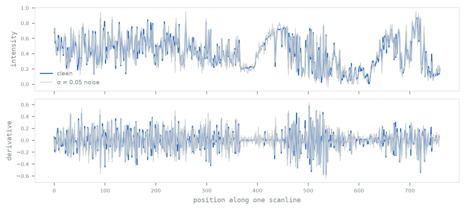
Finite differences have a problem, and Figure 1.16 shows it on one scanline of the scene. Add a little noise to the intensity profile and it stays recognisable; differentiate both, and the clean derivative is buried. Differentiation amplifies exactly what noise is made of: rapid small changes. The fix is to smooth before differentiating, and associativity collapses the two steps into convolution with a single kernel, the derivative of a Gaussian. One pass, and the noise-robustness of smoothing is built into the edge detector itself.

Figure 1.16: One scanline of the scene, clean and with mild noise. The intensity profiles (top) are nearly identical; their derivatives (bottom) are not — the noise, invisible in the signal, dominates its derivative.

1.4.2 The derivative kernels

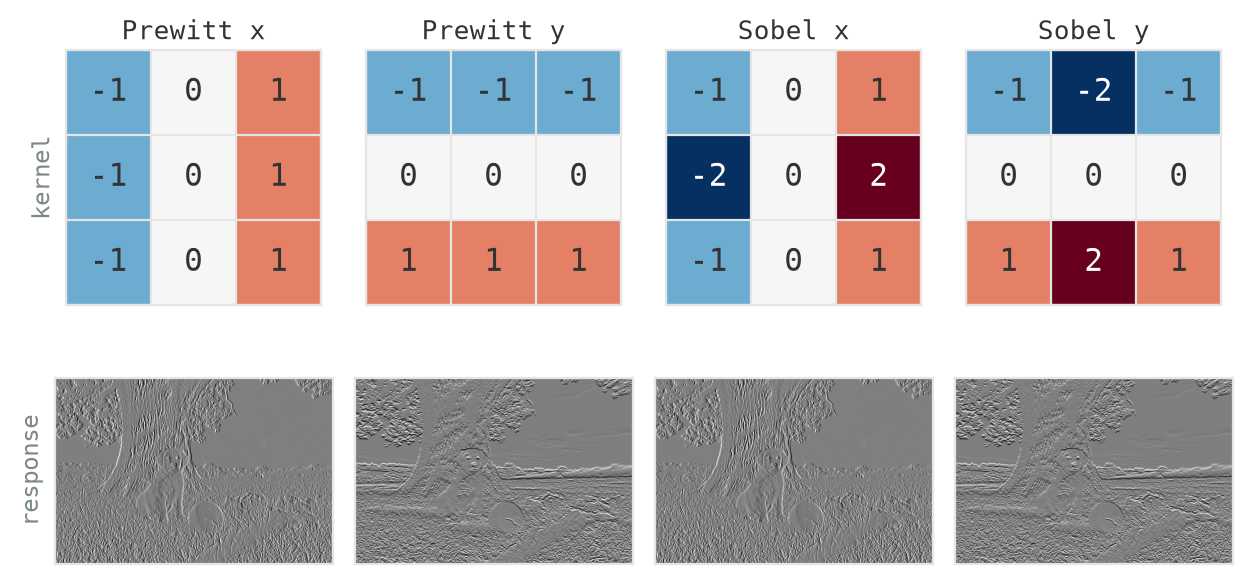
The estimators themselves are small enough to print, and worth reading as the tiny images they are. Prewitt’s pair is the bluntest useful design: a \([-1, 0, 1]\) difference in one direction, averaged with \([1, 1, 1]\) across the other, because Figure 1.16 has just shown what raw differencing does to noise. That \([-1, 0, 1]\) row is the central difference of numerical analysis, \(\bigl(I(x{+}1) - I(x{-}1)\bigr)/2\) up to its constant: symmetric about the pixel it scores, and accurate to second order, where the two-point \([-1, 1]\) that opened this section is first-order and lands its estimate halfway between pixels. Sobel doubles the centre of that average, giving \([1, 2, 1]\), one step toward a Gaussian, and became the default. Figure 1.17 shows both pairs at work. The responses are signed: mid-grey is zero, white a rise, black a fall, and each kernel responds only in its own direction. The \(x\) kernels pick out the trunk’s vertical edges and barely respond to the horizon; the \(y\) kernels do the reverse. On a photograph the two pairs are nearly indistinguishable, which is its own lesson: once some smoothing is present, the exact weights matter little.

Figure 1.17: First-derivative kernels and their responses on the scene. Prewitt differences in one direction and averages plainly across the other; Sobel doubles the centre of the average. Responses are signed: mid-grey is zero, white positive, black negative, each panel scaled to its own 99th percentile. The \(x\) kernels respond to vertical structure, the \(y\) kernels to horizontal, and the two pairs are nearly indistinguishable.

ImportantWhich way does an \(x\)-derivative look?

The naming trips everyone at least once. \([-1, 0, 1]\) differentiates along \(x\): it compares a pixel’s left neighbour with its right, within a row. A large response therefore means intensity changes as you move horizontally, and a place where intensity changes horizontally is a vertical edge. Its transpose, \([-1, 0, 1]^\mathsf{T}\), differentiates along \(y\), down a column, and so fires on horizontal edges. Check Figure 1.17 against this: the \(x\) responses draw the trunk’s sides, the \(y\) responses the horizon. A derivative kernel is named for the direction it differentiates, and the edges it finds run perpendicular to it.

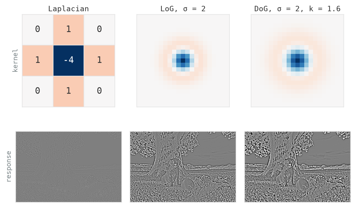
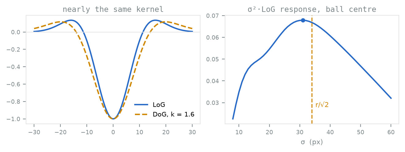
Second derivatives make the other classic family (Figure 1.18). The Laplacian sums the two unmixed second derivatives, \(\nabla^2 I = \partial^2 I/\partial x^2 + \partial^2 I/\partial y^2\), five integers as a kernel, and unlike a gradient it carries no direction: it responds where intensity curves, at spots, blobs, and both sides of every edge. Being a second derivative, it amplifies noise even more than the first, and its raw response on the scene is mostly speckle. The repair is the one this chapter keeps making: smooth first and fold the blur into the kernel, giving the Laplacian of Gaussian (LoG). And the LoG has a famous shortcut: subtract a Gaussian from a slightly wider one, and the resulting Difference of Gaussians (DoG) is nearly the same kernel, with the nearly identical response the figure shows. What a second-derivative filter is for, and why one would sweep its \(\sigma\), is the subject of Section 1.5.

ImportantWhere the five integers come from

Difference the differences. Write \(I_{i,j}\) for the pixel at column \(i\), row \(j\), take the two-point difference on either side of it along the row, and subtract one from the other:

\[ \frac{\partial^2 I}{\partial x^2}\bigg|_{i,j} \;\approx\; \underbrace{\bigl(I_{i+1,j} - I_{i,j}\bigr)}_{\text{difference on the right}} \;-\; \underbrace{\bigl(I_{i,j} - I_{i-1,j}\bigr)}_{\text{difference on the left}} \;=\; I_{i+1,j} - 2I_{i,j} + I_{i-1,j}, \]

the one-dimensional kernel \([1, -2, 1]\). Each two-point difference lands halfway between pixels; differencing the pair lands the estimate back on the pixel itself. The same construction down a column gives \([1, -2, 1]^\mathsf{T}\), and because the Laplacian is a sum of the two second derivatives, the kernels add, with the two \(-2\)s overlapping at the centre:

\[ \nabla^2 I \;\approx\; I_{i+1,j} + I_{i-1,j} + I_{i,j+1} + I_{i,j-1} - 4\,I_{i,j} \]

That is left, right, above and below, minus four times the centre: the kernel of Figure 1.18.

Figure 1.18: Second-derivative kernels and their responses on the scene. The discrete Laplacian is five integers and orientation-free, and its raw response is mostly noise, the lesson of Figure 1.16 compounded by the second derivative. The LoG folds the smoothing into the kernel. The DoG, a slightly wider Gaussian minus a narrower one, is nearly the same kernel and gives a nearly identical response.

1.4.3 Sobel: gradient magnitude and orientation

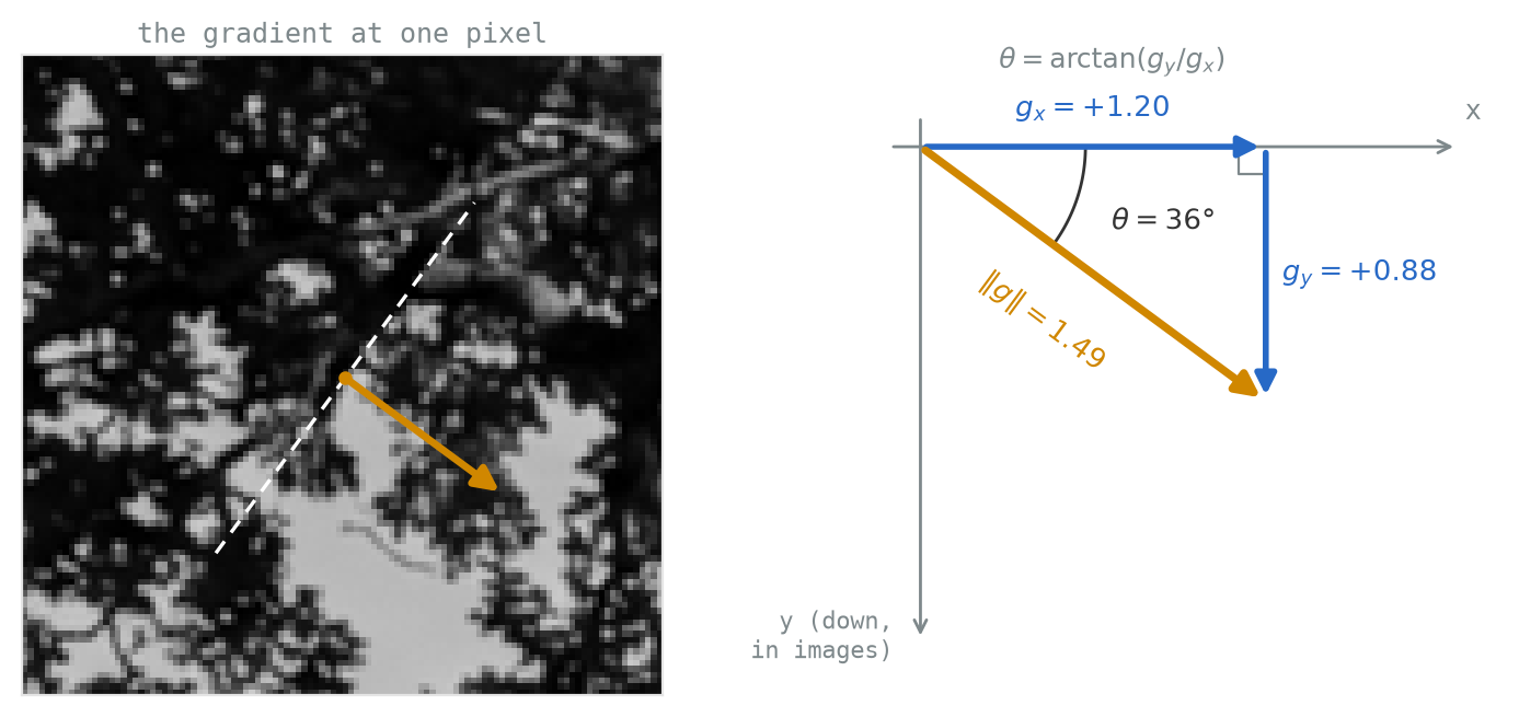
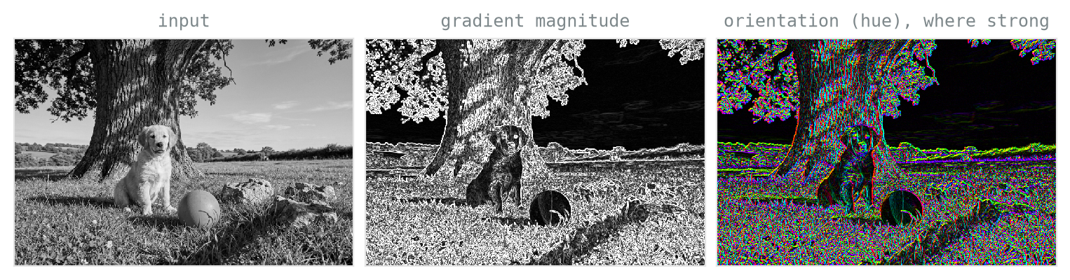
Stack the two Sobel responses of Figure 1.17 and every pixel carries the gradient \((g_x, g_y)\), and from it two numbers: the magnitude \(\sqrt{g_x^2 + g_y^2}\), which says how edge-like the pixel is, and the orientation \(\arctan(g_y / g_x)\), which says which way the edge faces. Figure 1.19 assembles the vector at a single pixel; Figure 1.20 then shows both numbers over the whole scene.

Figure 1.19: The gradient as a vector, at one pixel of a canopy edge. Left: the crop, with the measured gradient arrow pointing across the edge toward brighter, and the dashed line marking the edge itself, perpendicular to it. Right: the same numbers as a triangle: \(g_x = +1.20\), \(g_y = +0.88\), magnitude \(\sqrt{g_x^2 + g_y^2} = 1.49\), and \(\theta = \arctan(g_y/g_x) = 36°\). Gradients here are Sobel after a light blur (\(\sigma = 1.2\)), as Canny will do shortly. Image \(y\) runs downward, so positive \(\theta\) turns clockwise on the page.

The orientation matters later: histograms of gradient orientations over a patch are the core of both SIFT and HOG (Section 1.8).

Figure 1.20: Sobel gradients on the scene. Middle: gradient magnitude, bright where intensity changes fast. Right: gradient orientation shown as hue, only where the magnitude is strong.

1.4.4 Canny is a pipeline

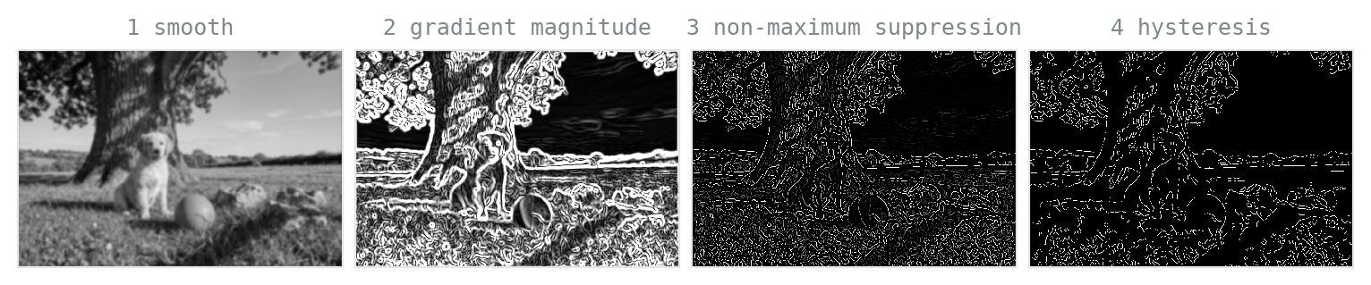
The Canny detector [1] is not one operation but four, each fixing a defect of the previous (Figure 1.21).

Smooth: a Gaussian blur sets the scale and gives noise-robustness. Gradient: Sobel gives magnitude everywhere, but “everywhere” is the problem, because edges come out thick. Non-maximum suppression: keep a pixel only if its magnitude beats its two neighbours along the gradient direction, so edges thin to one-pixel ridges. That move recurs; NMS, keeping the local best and deleting the runners-up, returns in object detection (Chapter 4). Hysteresis: two thresholds instead of one, where strong pixels survive and weak pixels survive only if connected to strong ones, so faint continuations of real contours are kept while isolated speckle is dropped.

Figure 1.21: The four Canny stages on the scene: smoothed input, gradient magnitude, the same after non-maximum suppression (edges thin to single-pixel ridges), and after hysteresis (weak but connected pixels kept, isolated ones dropped).

Interactive: the Canny pipeline

The four stages as tabs, with the parameters live at each one. Start with \(\sigma\), and notice it is doing more than suppressing noise: it sets the scale of edge the detector can find. At \(\sigma = 1\) every grass blade earns a contour; by \(\sigma = 4\) the blur has erased every boundary smaller than itself and only the trunk, the dog, the ball, and the horizon remain. The kernel zoo’s “structure much smaller than \(\sigma\) is gone” is now deciding which edges exist at all, and Section 1.5 builds a whole representation out of that dial. Then open the last tab, where the gold pixels are the ones hysteresis rescued: weak responses connected to something strong. Pull the two thresholds together and the rescue stops mattering; drop the low one and speckle comes back.

1.5 Scale and pyramids

A detector is matched to a pattern at one pixel size. The dog’s ear is thirty pixels across; the tree is three hundred. The same object also changes pixel size as it moves towards or away from the camera. Instead of building a detector for every possible size, we shrink the image and reuse one detector.

1.5.1 The Gaussian pyramid

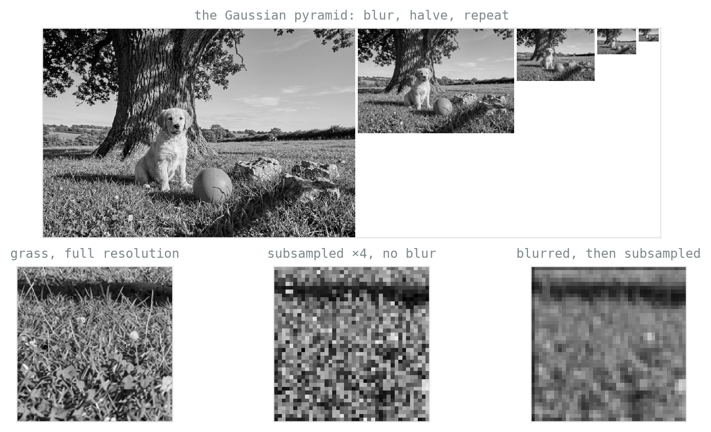
The Gaussian pyramid is the recipe from Section 1.1 applied recursively: blur, subsample by two, repeat (Figure 1.22). Each level is half the size. A ball 64 pixels wide in the original is 32 pixels wide at level 1 and 16 at level 2. A detector built for a 16-pixel ball can therefore find all three sizes by running unchanged at every level. Scale variation has become a search over levels.

Each halving also doubles what a fixed window spans in the original image. A \(3 \times 3\) kernel at level 2 covers the same area as a \(12 \times 12\) window in the original. The blur is not optional. Subsample the grass without blurring first and the fine blades reappear as false coarse clumps; blur first and the small levels are soft but truthful, exactly as the zone plate demonstrated.

Figure 1.22: Top: the Gaussian pyramid of the scene, blurring and halving repeatedly. Bottom: why the blur is mandatory. Subsampling the grass ×4 without it aliases the blades into false clumps; blurring first loses the detail honestly.

Interactive: one detector, every scale

The detector is fixed at \(24 \times 24\) pixels and expects a ball 16 pixels wide. Set the ball to 16 pixels, then double it. Before each click, predict which level will respond most strongly. The dashed box on the original shows how much of that image the winning detector spans.

1.5.2 The Laplacian pyramid

Subtract each pyramid level, upsampled back to size, from the one before it and you get the Laplacian pyramid [2]: each layer holds only the detail that lives between two scales: fine texture in \(L_0\), coarser structure in \(L_1\), and so on (Figure 1.23). The name is honorary, since no Laplacian is computed anywhere. Each layer is the same image blurred by two different amounts and subtracted, a difference of Gaussians, and Section 1.4.2 showed that a DoG is nearly the Laplacian-of-Gaussian filter: the pyramid is named for the operator its layers imitate, not one they apply.

NoteBuild and collapse

Write \(G_0\) for the image and fix a number of levels \(N\).

Build. For \(i = 0, 1, \dots, N-1\):

1. Blur \(G_i\) and subsample by two. The result is \(G_{i+1}\), the next Gaussian level.
2. Upsample \(G_{i+1}\) back to the size of \(G_i\); call the result \(\operatorname{up}(G_{i+1})\).
3. Subtract: \(L_i = G_i - \operatorname{up}(G_{i+1})\) — the detail the blur removed.

The bands \(L_0, \dots, L_{N-1}\), with the residual \(L_N = G_N\) on top, are the Laplacian pyramid.

Collapse. Start from the residual, \(R = L_N\), and for \(i = N-1\) down to \(0\) replace \(R\) with \(\operatorname{up}(R) + L_i\). The final \(R\) is \(G_0\) exactly, because each step adds back precisely the difference that step 3 removed: \(\operatorname{up}(G_{i+1}) + L_i = G_i\) by construction. The blur is never inverted, so any blur works — the only requirement is that the collapse upsample the same way the build did.

Nothing is lost: adding the layers back, coarsest to finest, reconstructs the image exactly. The classic demonstration is blending (Figure 1.23, bottom row). Join two images along a hard seam and the seam is all you see. Feather that seam with one soft mask and you trade the step for a ghost: across the whole transition, both textures are visible through each other, a double exposure a hand’s width wide. The repair is to blend each band with the mask blurred to that band’s scale — fine detail then changes over abruptly, so nothing ghosts, while brightness cross-fades over a wide region, so no step shows. The join becomes invisible.

ImportantBlending, step by step

Take two images, \(A\) and \(B\), and a binary mask \(M\) — 1 where \(A\) should win, 0 where \(B\) should.

1. Build a Laplacian pyramid of each image: \(L^A_i\) and \(L^B_i\).
2. Build a Gaussian pyramid of the mask: \(G^M_i\), at the same levels.
3. Blend level by level, pixel by pixel: \(L^C_i = G^M_i \, L^A_i + (1 - G^M_i)\, L^B_i\) — at each pixel, the blurred mask value says how much of \(A\)’s band survives.
4. Collapse \(L^C\) to get the blended image.

Step 2 is the whole trick, and it is why the mask gets a Gaussian pyramid rather than a Laplacian one. Each level is blurred in its own pixel units, so measured in original pixels the blend region doubles at every coarser level: in Figure 1.23 it runs 0, 4, 8, 16, and 32 pixels. Nobody chooses those widths; they fall out of the pyramid. Blur the mask once at full resolution instead and every band blends over the same width, which is the middle panel’s ghosting, not this algorithm.

Figure 1.23: Top: Laplacian levels of the scene, each holding the detail between two pyramid scales, shown around mid-grey. Bottom: joining bark to grass three ways. A hard seam leaves a visible step. One feather of fixed width leaves a ghost, with both textures showing through each other across the transition. Blending each band with the mask blurred to that band’s own scale leaves no join at all. Below, the mechanism: the mask’s Gaussian pyramid, each level’s profile plotted in original pixels; a hard step at level 0 doubles per level to a 32-pixel ramp at level 4, and nobody chose those widths.

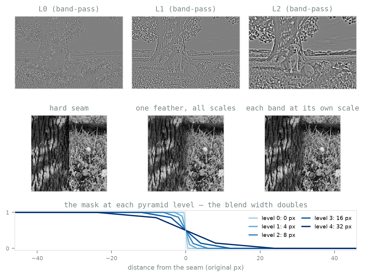
Interactive: blending, step by step

The recipe of the callout, one step at a time: the two textures and the mask, their pyramids, the mask’s widening levels, the per-band blend, and the collapse, watching the image assemble from its residual upward. Then the comparison. Two dials to try: drop levels to 1 and the join comes back, because with no coarse bands there is no wide cross-fade and the result heads toward the hard seam; then swap the mask for the circle or the diagonal, and drag the two crop boxes anywhere in the scene. The method does not depend on the mask’s shape or on what is being joined. Reset brings back bark against grass.

1.5.3 Scale space

A pyramid tells you what the scene looks like at each scale. It can also tell you which scale a given structure belongs to: how big the ball is in its own terms, not merely how many pixels wide it happens to be. The tool is the LoG of Section 1.4.2, run not once but across a range of \(\sigma\). One correction comes first. The Gaussian keeps its total weight fixed as it widens, so it flattens, and the LoG built on it responds ever more weakly as \(\sigma\) grows; left raw, it always answers loudest at the finest scale. Multiplying the response by \(\sigma^2\) cancels that decay and puts every scale on equal footing. The Laplacian has no preferred direction (Section 1.4.2): where Sobel faces one way, the LoG answers to an edge at every orientation at once, a closed ring rather than a straight step. Its sign flips across a circle of radius \(\sqrt{2}\,\sigma\), and that ring is the edge it is matched to, which makes the LoG a circular edge detector whose \(\sigma\) sets the radius it responds to. Sweep \(\sigma\) upward and the normalised response at a blob’s centre rises, peaks, and falls, peaking where the ring sits on the blob’s rim: for a disc of radius \(r\), at \(\sigma = r/\sqrt{2}\). A structure’s size is the \(\sigma\) at which it responds most strongly. Figure 1.24 runs this on the ball: its radius of 48 px (Figure 1.11) predicts a peak at \(\sigma \approx 34\), and the measured curve peaks at 31. The gap is because the ball is shaded and sits on textured grass rather than being a clean disc on a blank field.

The pyramid supplies the operator at almost no extra cost. Subtract two levels blurred by nearby amounts and you have a difference of Gaussians, and a DoG is nearly the LoG; Figure 1.24, left, overlays the two profiles at SIFT’s ratio \(k = 1.6\). Search a DoG stack for extrema across position and scale at once and you have how SIFT picks its keypoints (Section 1.8); the LoG itself returns as the blob filter of the MR8 bank (Section 1.7).

Figure 1.24: Scale selection at work. Left: radial cross-sections of the LoG and the DoG at ratio \(k = 1.6\) (SIFT’s choice), each scaled to unit centre, showing nearly the same profile. Right: the \(\sigma^2\)-normalised LoG response at the centre of the scene’s ball, across \(\sigma\): a clean disc of radius 48 would peak at \(\sigma = r/\sqrt{2} \approx 34\) (dashed); the measured peak sits at 31, pulled by the ball’s shading and the surrounding grass.

Pyramids return later, learned: as feature pyramid networks in detection (Chapter 4), and as the shrinking stages of hierarchical transformers (Chapter 9).

1.6 Noise, and how features die

Every sensor adds noise. The standard model is additive Gaussian noise: \[x_{ij} \leftarrow x_{ij} + \varepsilon,\] where \(\varepsilon \sim \mathcal{N}(0, \sigma^2)\) is sampled independently at each pixel.

1.6.1 The additive model

Against values in \([0,1]\), \(\sigma\) has direct meaning: at \(\sigma = 0.05\) a typical pixel is off by a twentieth of the full range, which is visible grain. The scene’s own intensities have a standard deviation near 0.25, so \(\sigma = 0.25\) is where the noise matches the signal’s spread and \(\sigma = 0.5\) is twice it. The signal-to-noise ratio is just that comparison made formal: signal power over \(\sigma^2\). The film strip below fixes six waypoints between clean image and pure static; every classical operation in this chapter lives somewhere on it.

Drag the slider and find the level at which edges stop being recoverable.

1.6.2 Watching edges die

The strip is a test bench, and Figure 1.25 puts the chapter’s edge detectors on it, each beside the kernel that defines it, with the film strip’s noise now a slider. Pick a detector, read it clean, then drag \(\sigma\) up. Which fails first? The raw Laplacian is barely holding on even at zero, since a second derivative on unsmoothed pixels is almost pure speckle, and the mildest noise finishes it, exactly as Figure 1.16 showed. The detectors that smooth before they differentiate (LoG, DoG, and Canny, whose first step is a blur) keep their edges far longer. Watch Canny in particular: at \(\sigma = 0.08\) the contours survive but speckle creeps in; by \(\sigma = 0.20\) real edges and noise edges are becoming hard to tell apart. In the lab you will do the same to SIFT matching and watch match counts collapse. The classical defence is the one this chapter keeps reaching for, which is to smooth more, and it costs precision: a bigger \(\sigma\) suppresses more noise and localises edges less precisely. You settle that trade-off once, when you choose \(\sigma\), and the choice is then applied unchanged to every image the pipeline will ever see, clean or noisy, fine-grained or coarse. The last section of the chapter is about what that rigidity costs.

Figure 1.25: The chapter’s edge detectors on the film strip, each beside its defining kernel, at any noise level. The raw Laplacian is almost pure speckle under the mildest noise; the detectors that smooth first, LoG, DoG and Canny, keep their edges far longer. Canny survives \(\sigma = 0.08\) with speckle creeping in, and by \(\sigma = 0.20\) its output is as much noise as signal.

1.7 Texture: Gabor, MR8, and textons

Edges find boundaries. Texture is what fills the regions between them, such as bark, grass and fur, and no single filter response captures it, because texture is not a value at a pixel but a statistic over a patch. The tools of this section all follow that logic: filter, then summarise the responses.

1.7.1 Gabor filters

A Gabor filter is a sinusoid under a Gaussian window: a small patch of oriented stripes that responds strongly where the image contains stripes of matching orientation and frequency (Figure 1.26). Three knobs, orientation, frequency and window size, sweep out a family of texture probes; the vertical grooves of the bark produce a strong response in the vertically-tuned filter and little in the others. The pattern is not arbitrary: the earliest cells of the visual cortex respond in strikingly Gabor-like ways, which is as far as this book will lean on the brain.

\[ g(x, y) = \underbrace{\exp\!\left(-\frac{x'^2 + y'^2}{2\sigma^2}\right)}_{\text{Gaussian window}}\; \underbrace{\cos\!\left(2\pi f x'\right)}_{\text{sinusoid}}, \]

where \(x' = x\cos\theta + y\sin\theta\) and \(y' = -x\sin\theta + y\cos\theta\) rotate the coordinates by the orientation \(\theta\), \(f\) sets the frequency, and \(\sigma\) the window size.

Figure 1.26: A small Gabor bank, two frequencies by four orientations, with one filter at work: the outlined, vertically-oriented, low-frequency filter responds strongly to the bark’s vertical grooves. Switch the widget to edit the values to steer orientation, frequency, and window size yourself and watch both the kernel and its response change.

NoteWhere the orientation tuning was first seen

Hubel and Wiesel found it by recording from a single cell in a cat’s visual cortex while sweeping a bar of light across its view: the cell fired for one orientation and fell silent for others. That is the observation the Gabor family imitates.

1.7.2 The MR8 filter bank

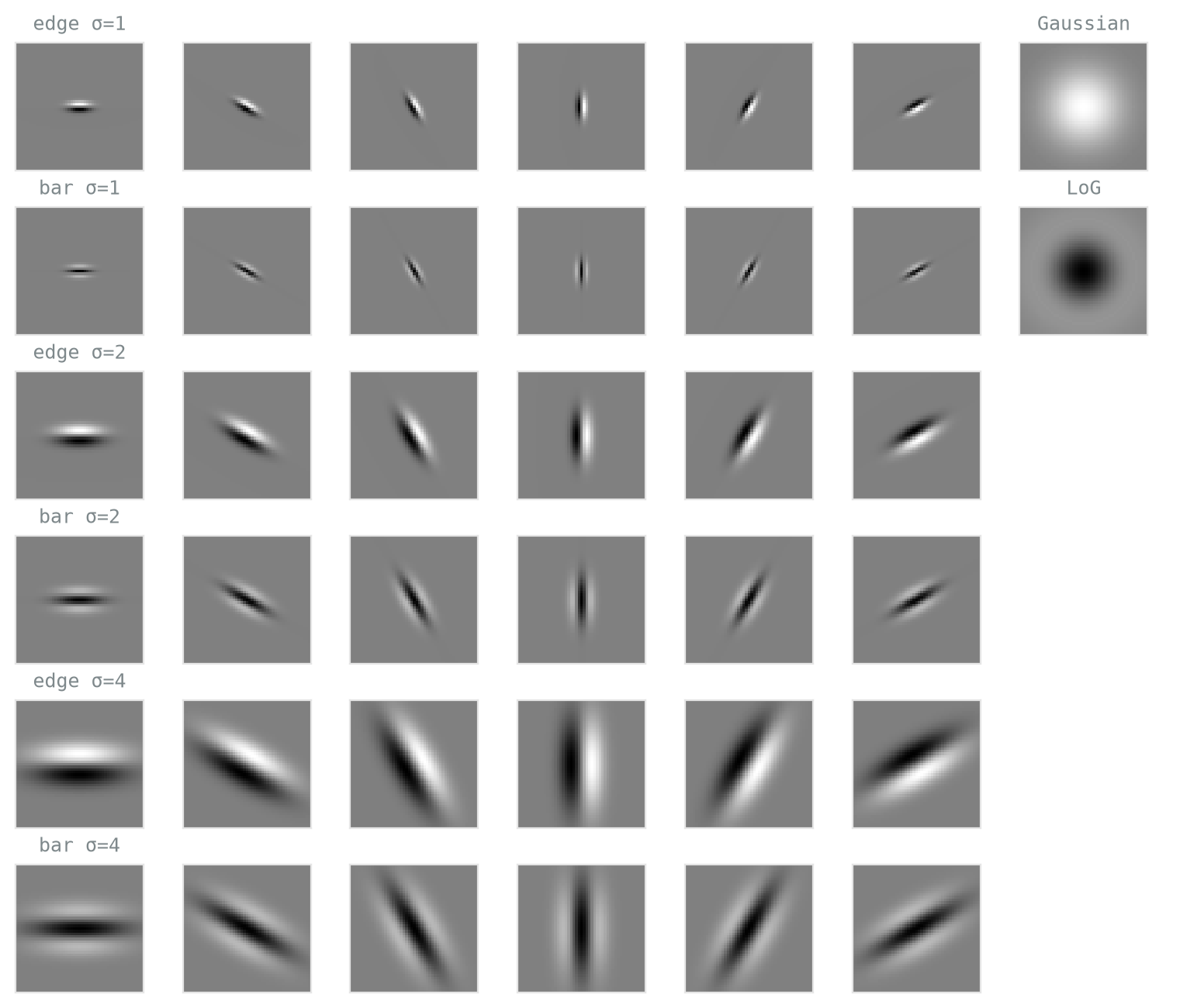
Texture classification wants coverage, so it uses a filter bank. The RFS bank behind MR8 [3] holds 38 filters: an edge filter and a bar filter at six orientations and three scales, plus a Gaussian and a Laplacian-of-Gaussian, the blob detector of Section 1.5 (Figure 1.27). The “MR” is maximum response: at each pixel, keep only the strongest response across the six orientations of each edge/bar-scale pair. Thirty-eight filters collapse to 8 channels, and the collapse gives invariance to in-plane rotation, since rotated bark excites a different orientation but the maximum over orientations is unchanged. Every part of this is a design choice, from the filter shapes to the six orientations, the three scales and the max, made by a person before any data arrives.

Figure 1.27: The RFS filter bank behind MR8: edge and bar filters at six orientations and three scales, plus a Gaussian and a Laplacian-of-Gaussian. Max-pooling each row of orientations collapses 38 filters to 8 responses.

1.7.3 Textons: cluster the responses

After MR8, every pixel carries an eight-dimensional response vector: how strongly each channel fired there. The vector is a compact description of the local structure around that pixel. Over a whole patch, the vectors form a cloud of points in eight-dimensional space. Bark’s cloud sits where the edge and bar channels are strong; grass’s sits where they are weaker and less oriented. The clouds overlap, but their dense regions do not, and those dense regions, the responses that recur, are what describe a texture.

k-means finds them. Fix the number of clumps, \(k\). Scatter \(k\) centres among the points, then repeat two steps until nothing moves: assign every point to its nearest centre, and move each centre to the mean of the points assigned to it. Assignment cuts the space into \(k\) cells; the move slides each centre to the middle of its cell; the next assignment redraws the cells around the shifted centres. A few passes and the centres settle on the cloud’s dense regions. Those settled centres are the textons [3], [4]: a small vocabulary of prototype responses, learned from the responses rather than chosen.

With the vocabulary fixed, describing a texture is bookkeeping. Assign each pixel to its nearest texton, and the image becomes a texton map, one label per pixel. Count how often each texton occurs and normalise, and the texture becomes a histogram over the vocabulary. The histogram is the texture’s signature, and it ignores where in the patch each texton fell. Two textures are compared by comparing histograms, with χ² distance or nearest-neighbour matching. Figure 1.28 runs the pipeline on the scene, with one comparison box on the trunk and one on the grass: the two histograms peak on different textons. That is the whole classifier, and it carried texture recognition for a decade.

Notek-means, formally

Given points \(\mathbf{x}_1, \dots, \mathbf{x}_n \in \mathbb{R}^d\) (here \(d = 8\)), k-means looks for \(k\) centres \(\boldsymbol{\mu}_1, \dots, \boldsymbol{\mu}_k\) and an assignment \(a(i)\) of each point to a centre that together minimise the within-cluster sum of squares, \[ J = \sum_{i=1}^{n} \bigl\lVert \mathbf{x}_i - \boldsymbol{\mu}_{a(i)} \bigr\rVert^2 . \] Lloyd’s algorithm descends \(J\) by alternating the two steps above. With the centres fixed, \(a(i) = \arg\min_c \lVert \mathbf{x}_i - \boldsymbol{\mu}_c \rVert\) is the assignment that minimises \(J\); with the assignment fixed, setting each \(\boldsymbol{\mu}_c\) to the mean of its members minimises it again. Each step lowers \(J\) or leaves it unchanged, so the iteration converges, though to a local minimum rather than necessarily the global one, which is why the starting centres matter and why k-means++ spreads them out before the first pass. One caveat: the distance is Euclidean, so each channel is standardised to unit variance first, or the highest-variance channel would dominate every comparison.

Figure 1.28: Textons on the scene. One vocabulary is clustered from the whole image’s MR8 responses, and the map colours each pixel by its nearest texton, so that bark, grass, fur, foliage, and sky land on different words. The two boxes read off their local histograms and the χ² separation between them; they start on the trunk and the grass. Drag them onto any other pair of textures, drop whole filter banks or single filters, and change \(k\): how few filters, and how small a vocabulary, keep χ² high? Every choice you make by hand here is one someone fixed for MR8, and one Chapter 2’s networks learn instead.

ImportantThe codebook recipe

Describe → cluster → assign → count. Extract local descriptors, cluster them into a finite vocabulary, assign each descriptor to its nearest word, and represent the whole image as a histogram of word counts. Textons apply it to filter responses. Bag of Visual Words, later this chapter, applies it to SIFT descriptors. Part of it returns when images become sequences of patch vectors (Chapter 9), and its assign step returns when those patches are given discrete codebook IDs to serve as training targets (Chapter 11).

1.8 Local features: Harris, SIFT, HOG

1.8.1 The matching problem

Take two photos of the same scene from different positions. To stitch them, or to recognise the scene again, you need to find the same physical point in both, which raises the question of what a point worth finding looks like. A flat patch is hopeless: it matches every other flat patch. An edge is little better: a window on an edge can slide along the edge without anything changing, so it matches everywhere along its own contour. What pins a location down in both directions is a corner, a place where the image changes whichever way you move.

1.8.2 Harris: corners from the structure tensor

Harris and Stephens [5] made “changes whichever way you move” computable, using the gradient images \(g_x\) and \(g_y\) of Section 1.4. Around each pixel, take a small window \(W\) and form the structure tensor, the Gaussian-weighted sum over the window of the products of the two gradients:

\[ M \;=\; \sum_{(x,y) \in W} w(x,y) \begin{bmatrix} g_x^2 & g_x g_y \\ g_x g_y & g_y^2 \end{bmatrix}, \]

where the weights \(w\) fall off from the window’s centre. Every entry is built from images the chapter already has, and the whole field costs five convolutions: two Sobel passes for the gradients, then a Gaussian blur of each of the three distinct products.

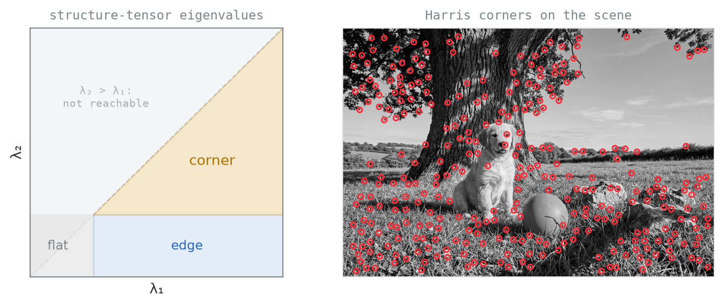
What the matrix means: slide the window a small step \((u, v)\) and compare it with itself. The summed squared difference grows as the quadratic form \(E(u,v) \approx \begin{bmatrix} u & v \end{bmatrix} M \begin{bmatrix} u \\ v \end{bmatrix}\), a bowl over the two shift directions, and the eigenvalues \(\lambda_1 \ge \lambda_2\) of \(M\) are the bowl’s curvatures along its principal axes. Figure 1.29 measures three windows of the scene. In the sky the bowl is a flat sheet: shift anywhere and nothing changes; both eigenvalues are near zero. On the trunk’s edge it is a valley, flat along the edge and steep across it, so one eigenvalue is large. At a rock corner it is a bowl with no flat direction, and both are large. The edge’s steep direction is in fact steeper than any direction of the corner’s bowl, so what makes a corner is the smallest curvature rather than the largest: \(\lambda_2\) measures the change along the direction that changes least, and only a corner keeps it large.

Figure 1.29: Three windows of the scene and, below each, the error surface \(E(u,v)\) of its measured structure tensor, showing how the summed squared difference grows as the window slides by \((u,v)\), with all three bowls on one vertical scale. Sky: a flat sheet, both eigenvalues near zero. Trunk edge: a valley, flat along the edge and steep across it. Rock corner: a bowl with no flat direction, both eigenvalues large. The dashed circle marks the Gaussian window (\(\sigma_w = 3.5\) px); gradients are Sobel after a \(\sigma = 1.2\) blur, as in Figure 1.19.

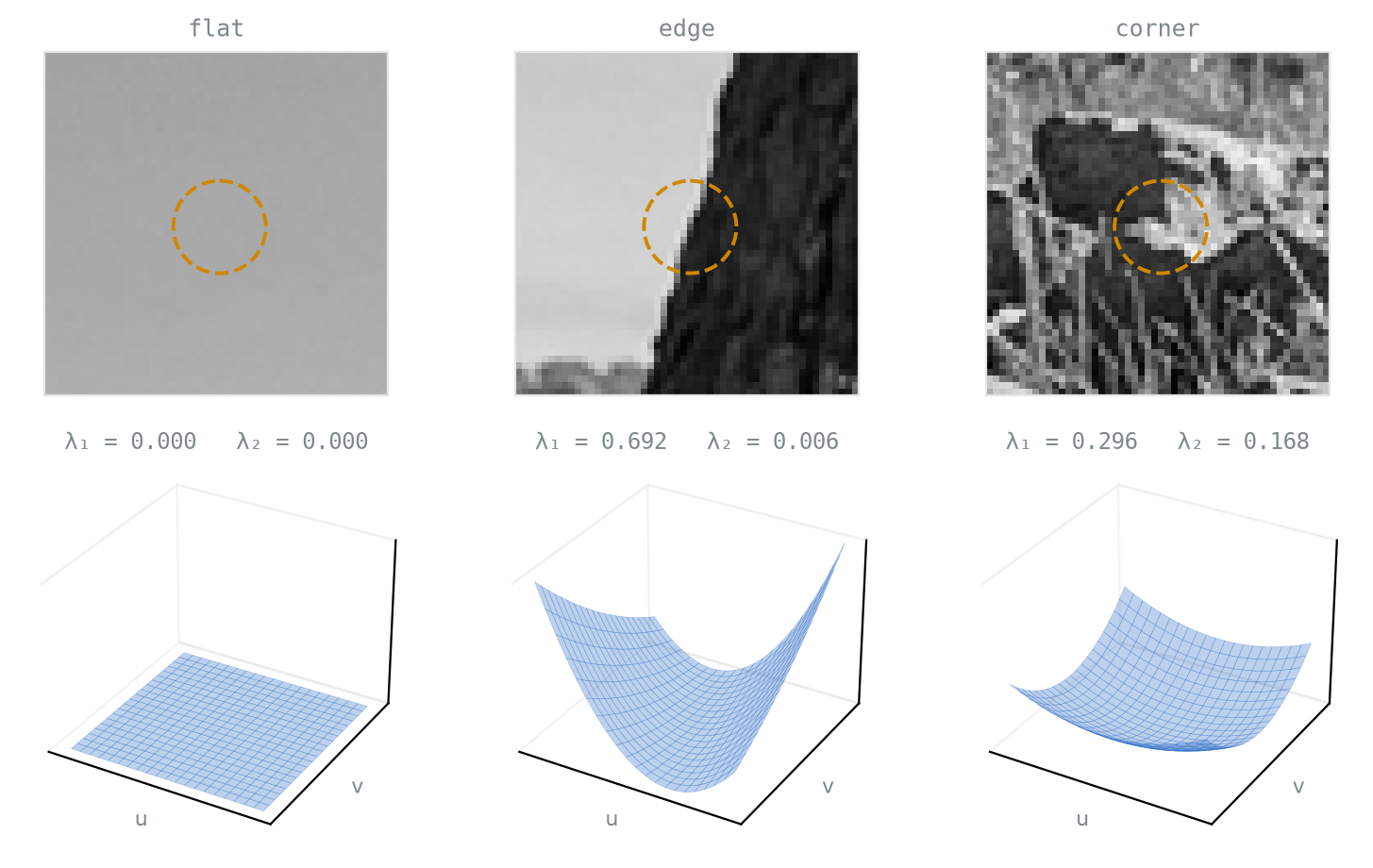
Figure 1.30, left, draws the resulting map of regimes in the \((\lambda_1, \lambda_2)\) plane. The Harris response folds the pair into one score, \(R = \det M - \kappa \, (\operatorname{tr} M)^2\) with \(\kappa \approx 0.05\). Since \(\det M = \lambda_1 \lambda_2\) and \(\operatorname{tr} M = \lambda_1 + \lambda_2\), \(R\) is large only where both eigenvalues are, with no eigendecomposition ever computed. Its peaks (right panel) land where you would put your finger: rock edges, branch forks, the dog’s features, and nothing at all in the sky. The grass is the warning: dense texture is corners everywhere, a reminder that “distinctive” is relative to what surrounds it.

Figure 1.30: Left: the eigenvalue picture of the structure tensor, showing the flat, edge, and corner regimes. Right: Harris corner peaks on the scene; the flat sky yields none, while structured regions and texture fire freely.

Interactive: the structure tensor

Drag the window. The middle panel shows the window’s gradients as a cloud with the tensor’s ellipse over them; the right panel is the eigenvalue plane from Figure 1.30 with your window as the moving point. Sky, edge, corner — then grass, and decide what “corner” means there.

1.8.3 SIFT: scale, orientation, descriptor

A corner detector answers where; matching also needs a description of what the neighbourhood looks like, stable under the ways a second photo differs from the first. SIFT [6] builds both, in three steps.

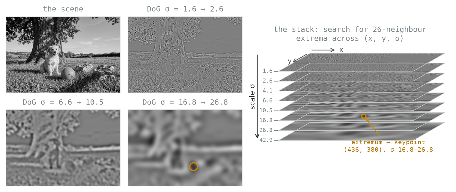
Where, and at what size. Build the difference-of-Gaussians stack of Section 1.5 and search it for extrema across position and scale at once: a keypoint is a pixel whose DoG value beats all 26 of its neighbours, the 8 around it in its own level and the 9 in each of the levels one scale below and above. Beating its own level finds where; beating the levels beside it finds at which scale. That is the scale selection of Section 1.5 run at every pixel at once, so each keypoint arrives with its own size attached. Extrema that sit on edges rather than corners are discarded by a Harris-style ratio test on the local curvatures, since an edge slides along itself and a point that slides cannot be matched. Figure 1.31 runs the search on the scene.

Figure 1.31: Scale selection run as a volume search. Left: the scene and three of its eight difference-of-Gaussians slices, blurs a factor \(k = 1.6\) apart. Right: all eight slices stacked over \((x, y, \sigma)\), each labelled with the finer of its two blurs. The strongest 26-neighbour extremum near the ball (gold) sits at \((436, 380)\) in the \(\sigma = 16.8 \to 26.8\) slice; full SIFT, with finer scale steps and sub-voxel interpolation, localises the same keypoint to \((435, 381)\) at \(\sigma = 18.9\). That is the keypoint whose descriptor Figure 1.32 builds.

Which way up. Around the keypoint, at its scale, histogram the gradient orientations of the neighbourhood into 36 bins, each vote weighted by the gradient’s magnitude and by closeness to the centre. The peak of that histogram becomes the keypoint’s orientation. Click a keypoint in the widget’s last tab and this histogram is what appears.

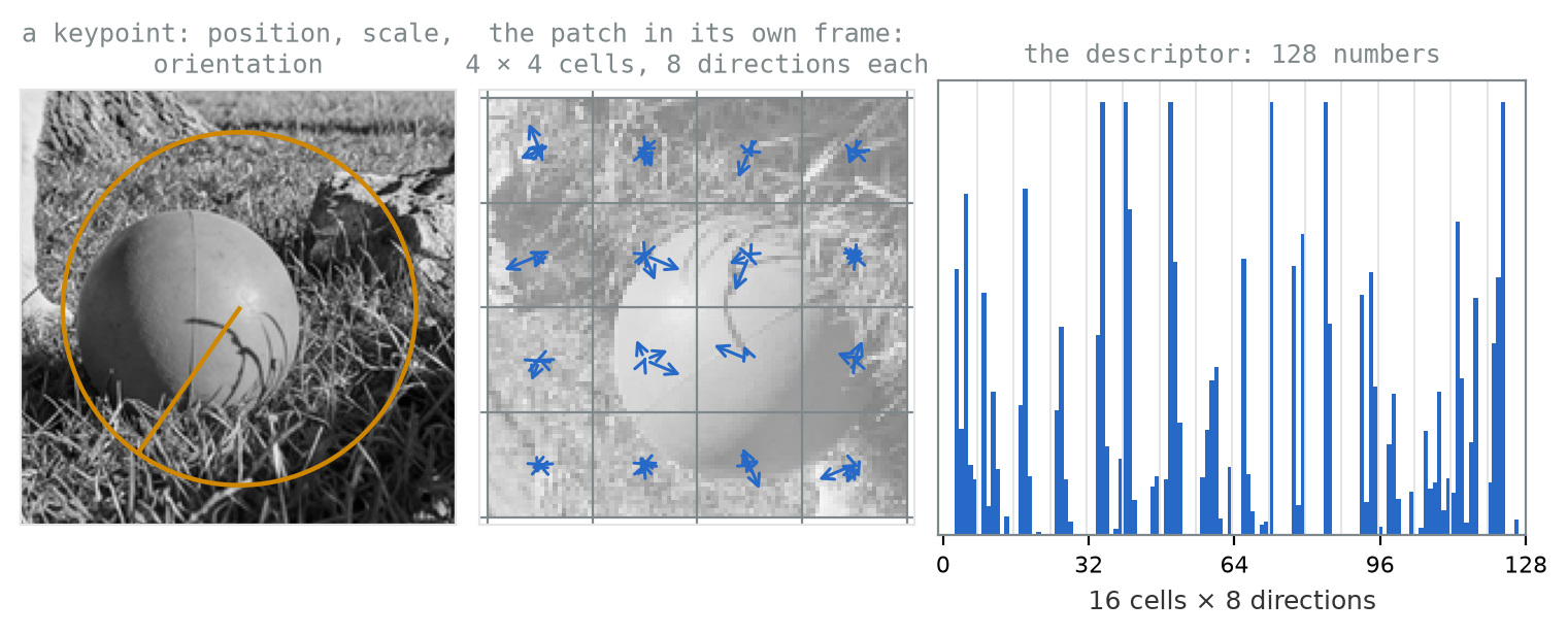
What. Sample a \(16 \times 16\) grid of gradients around the keypoint, at its scale and rotated to its orientation, so the patch is measured in the keypoint’s own coordinates. Divide the grid into \(4 \times 4\) cells, give each cell an 8-bin histogram of gradient direction, and concatenate: \(4 \times 4 \times 8 = 128\) numbers. Normalise the vector so uniform lighting changes cancel. Figure 1.32 builds one, for the keypoint SIFT finds on the ball. Two keypoints match when their descriptors are nearest neighbours, and the match is kept only if it is clearly better than the second-best candidate, the ratio test the lab uses.

Figure 1.32: The descriptor, built for one real keypoint: the one SIFT finds on the ball, with its scale and orientation drawn at left. Middle: the patch resampled in the keypoint’s own frame, rotated to its orientation and sized to its scale, with each of the \(4 \times 4\) cells drawn as its eight direction arrows, length proportional to that bin’s weight. Right: the same numbers flattened into the 128-vector that is matched between images. Computed as the text describes: \(16 \times 16\) gradient samples, centre-weighted, binned by direction, normalised and clipped.

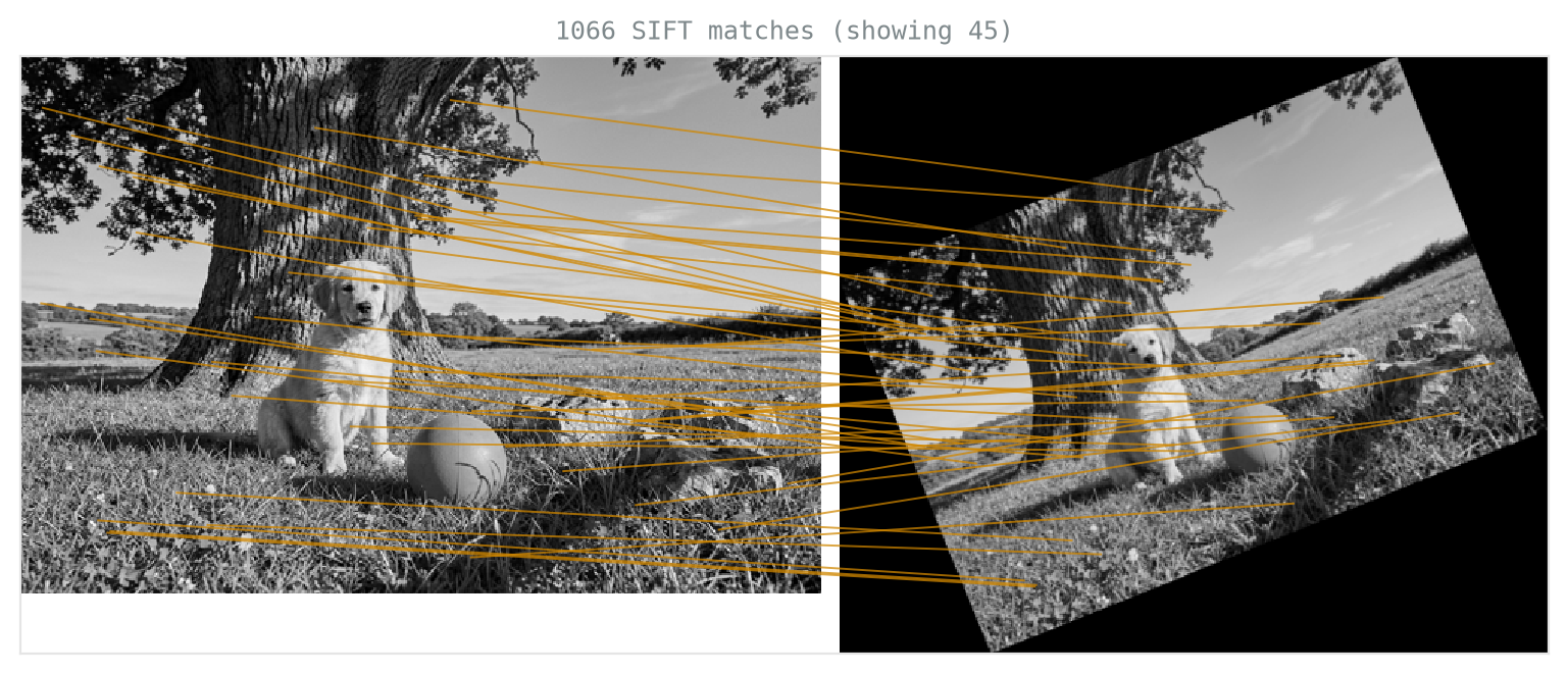
The result is invariant to translation, rotation, and scale, and robust to modest lighting change. None of it holds under large viewpoint change or occlusion. Figure 1.33 shows the machinery working across a rotation and a rescale that would defeat raw patch comparison; in the lab, you will watch the same match counts collapse as the film strip’s noise rises.

A descriptor summarising a small patch, computed at many locations. Keep the shape of that idea; we will meet it again (Chapter 9).

Figure 1.33: SIFT matches between the scene and a rotated, rescaled copy. Each line connects a keypoint to its matched partner; descriptor matching survives a transformation that would defeat direct patch comparison.

Interactive: SIFT, stage by stage

The four stages as tabs: blur stack, difference of Gaussians, the 26-neighbour extrema test, and finally every keypoint with its scale and orientation. In the last tab, click a keypoint to see the orientation histogram that chose its arrow.

1.8.4 HOG: dense description

SIFT describes a sparse set of chosen points. HOG [7] drops the choosing and describes the whole window, in three steps.

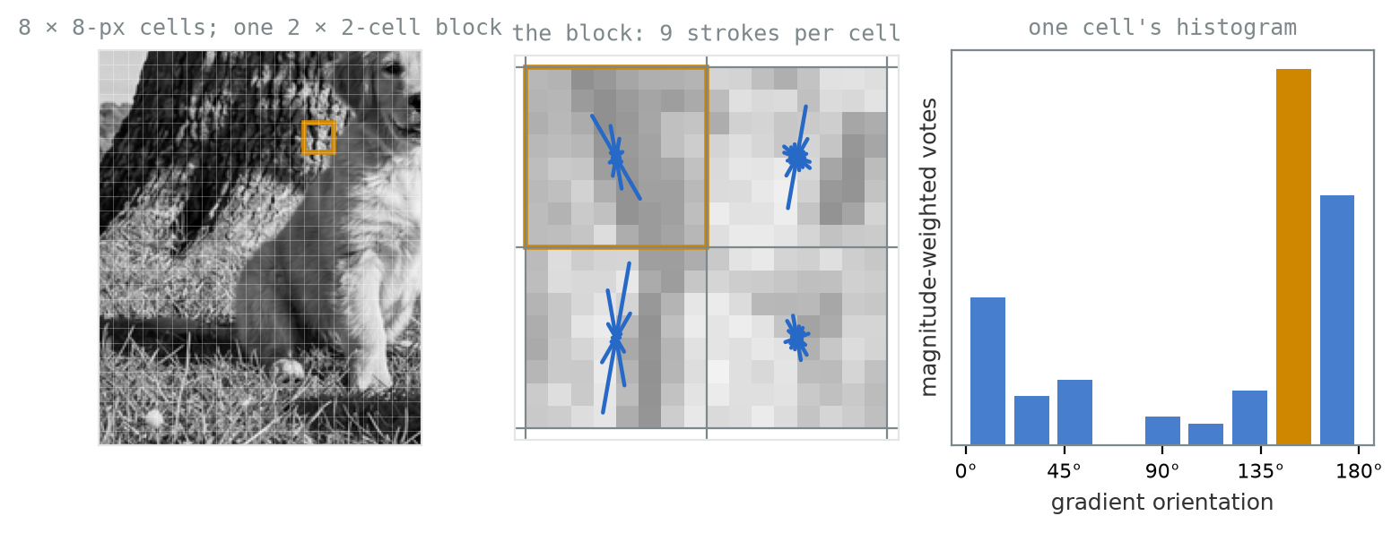
Cells. Divide the window into cells of \(8 \times 8\) pixels. Each cell gets a 9-bin histogram of gradient orientation over 0–180°, unsigned so that a dark-to-light edge and a light-to-dark edge vote alike, with every pixel’s vote weighted by its gradient magnitude. One cell becomes 9 numbers: which ways the edges run there, and how strongly.

Blocks. Gradient magnitudes rise and fall with the lighting. So group \(2 \times 2\) neighbouring cells into a block, normalise the block’s \(36\) numbers to unit length, and slide the block along one cell at a time, so every cell is re-normalised against up to four different neighbourhoods. Local contrast cancels; the orientations survive. Figure 1.34 shows one block of the dog crop: the four cells, the nine strokes of each with length proportional to that bin’s votes, and one cell’s histogram as bars.

Figure 1.34: The HOG construction, zoomed. Left: the crop divided into \(8 \times 8\)-pixel cells, one \(2 \times 2\)-cell block boxed. Middle: that block enlarged, each cell drawn as nine strokes, one per orientation bin, length proportional to the bin’s magnitude-weighted votes; the strokes run along the structure that produced them. Right: the outlined cell’s histogram as bars, the nine numbers HOG keeps for that cell.

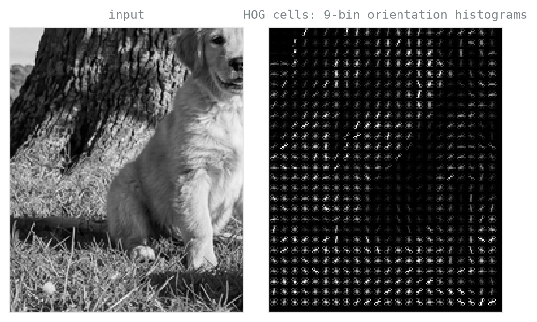
One long vector. Concatenate every block. For the classic \(64 \times 128\) pedestrian window that is \(8 \times 16\) cells, \(7 \times 15\) overlapping blocks, and \(7 \times 15 \times 4 \times 9 = 3780\) numbers (Figure 1.35 shows the cell histograms as oriented strokes). No keypoints, and no invariances beyond the normalisation: just a dense summary of which way local structure runs, everywhere. Slide the window across the image and hand each vector to a linear classifier, and you have the detector that first made pedestrian detection work.

Sparse description for matching points; dense description for recognising layouts. Both are gradient-orientation histograms underneath.

Figure 1.35: HOG on the dog: each \(8 \times 8\)-pixel cell is summarised by a 9-bin histogram of gradient orientations, drawn as oriented strokes. The dog’s outline survives as a pattern of dominant orientations.

1.9 Bag of Visual Words

1.9.1 The recipe, second serving

To classify whole images, apply the codebook recipe again, this time with SIFT descriptors as the raw material [8]. Extract descriptors (at keypoints, or on a dense grid); cluster a training sample of them with k-means into a vocabulary of visual words, whose size is a knob someone must turn, a hyperparameter, as the textons’ \(k\) already was; assign every descriptor in an image to its nearest word; and represent the image as the normalised histogram of word counts. A linear SVM or k-NN on the histograms completes the classifier. Set the two servings side by side:

Table 1.1: One recipe, two servings.

	descriptor	vocabulary	document
Textons	MR8 responses, every pixel	8–64 textons	a texture patch
Bag of Visual Words	SIFT, at keypoints	200–10,000 words	a whole image

1.9.2 What the histogram throws away

Everything spatial. A dog above grass and grass above a dog produce identical histograms; the representation knows what is in the image and nothing about where. The standard patch is spatial pyramid matching [9]: histogram the whole image, then its quarters, then sixteenths, and concatenate. Coarse layout re-enters and accuracy rises accordingly. It is a patch, though, not a cure, and where returns as the central question of Part II.

1.9.3 Where this got the field

Far, and then no further. With spatial pyramids, BoVW-family systems reached about 65% on Caltech-101 in 2006 [9], and refinements pushed the ImageNet challenge’s best top-5 error to roughly 26% by 2011, the strongest results hand-crafted features ever produced. A decade of accumulated craft went into better descriptors, better codebooks and better kernels, and each year’s gain was smaller than the last. What happened to that 26% in 2012 opens Chapter 2.

1.10 The ceiling: what hand-crafting cannot do

Inventory the pipeline this chapter built. Gaussian \(\sigma\): chosen. Sobel weights: chosen. Canny’s thresholds: chosen. The MR8 bank’s shapes, orientations, and scales: chosen. SIFT’s \(4 \times 4 \times 8\) grid, HOG’s cell size, the vocabulary’s word count: chosen, chosen, chosen. Every stage was designed by a person, fixed before any data arrived, and then applied identically to every image and every task.

That is the ceiling. Nothing in MR8 knows whether the task is telling bark from brick or finding pedestrians in fog; the features cannot adapt to what the problem actually needs, and the only way to improve them is for a human to think of something better. For a decade, humans did — and the curve of those improvements flattened all the same, stalling near that 26% on ImageNet while each year’s cleverness bought less than the last.

Here is the question the next chapter answers. The first thing MR8 does to an image is apply a bank of small oriented filters. The first thing the network you will meet next week does to an image is also apply a bank of small oriented filters — and when you look at that network’s filters, learned from data with no human guidance, they look uncannily like the bank you just met: oriented edges, bars, and blobs. Nobody designed them. That is the entire difference.

Where do benchmark images come from? The retraction of Tiny Images and several face datasets is a short, instructive history: scale was achieved by scraping people who never consented [10].

Exercises

1. Pinhole geometry. A pinhole camera with \(f = 50\) mm images a person 1.8 m tall standing 10 m away. How tall is their image on the sensor, and which way up? What happens to the image if you double \(f\)? If you double the pinhole diameter instead?
2. Reading transfer curves. Sketch the transfer function \(f(v)\) for: (a) brightness +50 on uint8, (b) contrast doubled about the midpoint, (c) \(\gamma = 0.5\), (d) histogram equalisation of an underexposed image (the general shape — the exact curve depends on the image’s histogram). For each, state what happens at the extremes of the range and what information, if any, is destroyed.
3. Colour space choice. You must segment a yellow robot ball under changing indoor lighting. Explain why a threshold box in RGB fails as lighting varies, and which HSV channel(s) you would threshold instead. When does the hue channel itself become unreliable?
4. Output sizes. An image is \(224 \times 224\). You convolve with a \(7 \times 7\) kernel, stride 2, padding 3. What size is the output? Now do it symbolically — and keep the formula; you will use it weekly from Chapter 2 on.
5. Separability. Show that a 2D Gaussian kernel factors into two 1D convolutions, and count multiplications per pixel for \(k = 31\) in both forms. What property of the box filter makes it separable too?
6. Flip or no flip. Give a kernel for which correlation and convolution produce different outputs, and one for which they cannot. What does this imply for the Sobel-\(x\) filter?
7. Canny reasoning. Before running anything, predict what happens to Canny output as (a) blur σ increases with thresholds fixed, and (b) the two hysteresis thresholds are moved toward each other. Verify with the widget.
8. Aliasing. Why must a Gaussian pyramid blur before subsampling? Construct (on paper) a 1D signal that demonstrates the failure if you skip the blur.
9. Invariance audit. For each of the Harris response map, the SIFT descriptor, and an MR8 texton histogram, state whether the representation is invariant, equivariant, or neither with respect to: translation, rotation, uniform scaling, and additive brightness change. Treat each transformation as ideal: no clipping, no boundary or resampling effects. Justify each cell in one sentence.
10. One recipe, two dishes. Write the codebook recipe as four steps. Fill in what plays the role of “descriptor”, “vocabulary”, and “document” for textons and for BoVW. What information does the final histogram discard in both cases, and name one task where that loss is fatal.
11. Robustness curve. Using the film-strip from the lab, plot Canny precision against the clean edges (the lab’s metric) — or the number of surviving SIFT matches — against noise σ. At what σ does the curve collapse, and does smoothing more delay the collapse — at what cost?

Lab 1: Convolution and classical filtering

Lab 1: point-op warm-up (gamma, contrast stretch, histogram equalisation as NumPy one-liners); convolution, blur, and edges from scratch in NumPy; the noise film-strip, then Canny and SIFT matching run across it to measure degradation; Gabor/MR8 textons and BoVW as one codebook exercise. CPU-only.

Open in Colab

Further reading

• Szeliski [11], chapters 3–4 — the reference treatment of filtering, pyramids, and features; free online.
• Canny [1] — the edge-detection pipeline as a designed artifact, worth skimming for how explicitly each stage is justified.
• Lowe [6] — SIFT; still one of the most cited papers in the field’s history.
• Dalal and Triggs [7] — HOG; a masterclass in careful feature engineering and ablation.
• Varma and Zisserman [3] — MR8 and texton classification; the codebook recipe at full strength.
• Csurka et al. [8] and Lazebnik et al. [9] — Bag of Visual Words and its spatially-aware fix.
• Birhane and Prabhu [10] — the dataset-provenance reading behind this chapter’s ethics card.

References

[1]

R. Szeliski, Computer vision: Algorithms and applications, 2nd ed. Springer, 2022. Available: https://szeliski.org/Book/

[2]

J. Canny, “A computational approach to edge detection,” IEEE Transactions on Pattern Analysis and Machine Intelligence, vol. 8, no. 6, pp. 679–698, 1986, doi: 10.1109/TPAMI.1986.4767851.

[3]

C. Harris and M. Stephens, “A combined corner and edge detector,” in Proceedings of the alvey vision conference, 1988, pp. 147–151. doi: 10.5244/C.2.23.

[4]

P. J. Burt and E. H. Adelson, “The Laplacian pyramid as a compact image code,” IEEE Transactions on Communications, vol. 31, no. 4, pp. 532–540, 1983, doi: 10.1109/TCOM.1983.1095851.

[5]

D. G. Lowe, “Distinctive image features from scale-invariant keypoints,” International Journal of Computer Vision, vol. 60, no. 2, pp. 91–110, 2004, doi: 10.1023/B:VISI.0000029664.99615.94.

[6]

N. Dalal and B. Triggs, “Histograms of oriented gradients for human detection,” in IEEE conference on computer vision and pattern recognition (CVPR), 2005, pp. 886–893. doi: 10.1109/CVPR.2005.177.

[7]

T. Leung and J. Malik, “Representing and recognizing the visual appearance of materials using three-dimensional textons,” International Journal of Computer Vision, vol. 43, no. 1, pp. 29–44, 2001, doi: 10.1023/A:1011126920638.

[8]

M. Varma and A. Zisserman, “A statistical approach to texture classification from single images,” International Journal of Computer Vision, vol. 62, no. 1–2, pp. 61–81, 2005, doi: 10.1007/s11263-005-4635-4.

[9]

G. Csurka, C. R. Dance, L. Fan, J. Willamowski, and C. Bray, “Visual categorization with bags of keypoints,” in ECCV workshop on statistical learning in computer vision, 2004. Available: https://www.cs.cmu.edu/~efros/courses/LBMV07/Papers/csurka-eccv-04.pdf

[10]

S. Lazebnik, C. Schmid, and J. Ponce, “Beyond bags of features: Spatial pyramid matching for recognizing natural scene categories,” in IEEE conference on computer vision and pattern recognition (CVPR), 2006, pp. 2169–2178. doi: 10.1109/CVPR.2006.68.

[11]

Y. LeCun, L. Bottou, Y. Bengio, and P. Haffner, “Gradient-based learning applied to document recognition,” Proceedings of the IEEE, vol. 86, no. 11, pp. 2278–2324, 1998, doi: 10.1109/5.726791.

[12]

K. Fukushima, “Neocognitron: A self-organizing neural network model for a mechanism of pattern recognition unaffected by shift in position,” Biological Cybernetics, vol. 36, no. 4, pp. 193–202, 1980, doi: 10.1007/BF00344251.

[13]

A. Krizhevsky, I. Sutskever, and G. E. Hinton, “ImageNet classification with deep convolutional neural networks,” in Advances in neural information processing systems (NIPS), 2012, pp. 1097–1105.

[14]

O. Russakovsky et al., “ImageNet large scale visual recognition challenge,” International Journal of Computer Vision, vol. 115, no. 3, pp. 211–252, 2015, doi: 10.1007/s11263-015-0816-y.

[15]

M. D. Zeiler and R. Fergus, “Visualizing and understanding convolutional networks,” in European conference on computer vision (ECCV), 2014, pp. 818–833. doi: 10.1007/978-3-319-10590-1_53.

[16]

K. Simonyan and A. Zisserman, “Very deep convolutional networks for large-scale image recognition,” in International conference on learning representations (ICLR), 2015. Available: https://arxiv.org/abs/1409.1556

[17]

C. Szegedy et al., “Going deeper with convolutions,” in IEEE conference on computer vision and pattern recognition (CVPR), 2015, pp. 1–9. doi: 10.1109/CVPR.2015.7298594.

[18]

S. Ioffe and C. Szegedy, “Batch normalization: Accelerating deep network training by reducing internal covariate shift,” in International conference on machine learning (ICML), 2015, pp. 448–456.

[19]

S. Santurkar, D. Tsipras, A. Ilyas, and A. Mądry, “How does batch normalization help optimization?” in Advances in neural information processing systems (NeurIPS), 2018, pp. 2483–2493.

[20]

D. P. Kingma and J. Ba, “Adam: A method for stochastic optimization,” in International conference on learning representations (ICLR), 2015. Available: https://arxiv.org/abs/1412.6980

[21]

A. Pretorius et al., “If dropout limits trainable depth, does critical initialisation still matter? A large-scale statistical analysis on ReLU networks,” Pattern Recognition Letters, vol. 138, pp. 95–105, 2020, doi: 10.1016/j.patrec.2020.06.025.

[22]

K. He, X. Zhang, S. Ren, and J. Sun, “Delving deep into rectifiers: Surpassing human-level performance on ImageNet classification,” in IEEE international conference on computer vision (ICCV), 2015, pp. 1026–1034. doi: 10.1109/ICCV.2015.123.

[23]

K. He, X. Zhang, S. Ren, and J. Sun, “Deep residual learning for image recognition,” in IEEE conference on computer vision and pattern recognition (CVPR), 2016, pp. 770–778. doi: 10.1109/CVPR.2016.90.

[24]

K. He, X. Zhang, S. Ren, and J. Sun, “Identity mappings in deep residual networks,” in European conference on computer vision (ECCV), 2016, pp. 630–645. doi: 10.1007/978-3-319-46493-0_38.

[25]

S. Xie, R. Girshick, P. Dollár, Z. Tu, and K. He, “Aggregated residual transformations for deep neural networks,” in IEEE conference on computer vision and pattern recognition (CVPR), 2017, pp. 1492–1500. doi: 10.1109/CVPR.2017.634.

[26]

A. G. Howard et al., “MobileNets: Efficient convolutional neural networks for mobile vision applications,” arXiv preprint arXiv:1704.04861, 2017, Available: https://arxiv.org/abs/1704.04861

[27]

M. Tan and Q. V. Le, “EfficientNet: Rethinking model scaling for convolutional neural networks,” in International conference on machine learning (ICML), 2019, pp. 6105–6114.

[28]

M. Lin, Q. Chen, and S. Yan, “Network in network,” in International conference on learning representations (ICLR), 2014. Available: https://arxiv.org/abs/1312.4400

[29]

N. Srivastava, G. Hinton, A. Krizhevsky, I. Sutskever, and R. Salakhutdinov, “Dropout: A simple way to prevent neural networks from overfitting,” Journal of Machine Learning Research, vol. 15, pp. 1929–1958, 2014, Available: https://jmlr.org/papers/v15/srivastava14a.html

[30]

R. Zhang, “Making convolutional networks shift-invariant again,” in International conference on machine learning (ICML), 2019, pp. 7324–7334.

[31]

V. Dumoulin and F. Visin, “A guide to convolution arithmetic for deep learning,” arXiv preprint arXiv:1603.07285, 2016, Available: https://arxiv.org/abs/1603.07285

[32]

A. Odena, V. Dumoulin, and C. Olah, “Deconvolution and checkerboard artifacts,” Distill, 2016, doi: 10.23915/distill.00003.

[33]

W. Luo, Y. Li, R. Urtasun, and R. Zemel, “Understanding the effective receptive field in deep convolutional neural networks,” in Advances in neural information processing systems (NIPS), 2016, pp. 4898–4906.

[34]

J. Donahue et al., “DeCAF: A deep convolutional activation feature for generic visual recognition,” in International conference on machine learning (ICML), 2014, pp. 647–655.

[35]

A. S. Razavian, H. Azizpour, J. Sullivan, and S. Carlsson, “CNN features off-the-shelf: An astounding baseline for recognition,” in IEEE conference on computer vision and pattern recognition workshops (CVPRW), 2014, pp. 806–813. doi: 10.1109/CVPRW.2014.131.

[36]

J. Yosinski, J. Clune, Y. Bengio, and H. Lipson, “How transferable are features in deep neural networks?” in Advances in neural information processing systems (NIPS), 2014, pp. 3320–3328.

[37]

R. Geirhos, P. Rubisch, C. Michaelis, M. Bethge, F. A. Wichmann, and W. Brendel, “ImageNet-trained CNNs are biased towards texture; increasing shape bias improves accuracy and robustness,” in International conference on learning representations (ICLR), 2019. Available: https://arxiv.org/abs/1811.12231

[38]

K. He, R. Girshick, and P. Dollár, “Rethinking ImageNet pre-training,” in IEEE international conference on computer vision (ICCV), 2019, pp. 4918–4927. doi: 10.1109/ICCV.2019.00502.

[39]

I. Goodfellow, Y. Bengio, and A. Courville, Deep learning. MIT Press, 2016. Available: https://www.deeplearningbook.org/

[40]

A. Birhane and V. U. Prabhu, “Large image datasets: A pyrrhic win for computer vision?” in IEEE winter conference on applications of computer vision (WACV), 2021, pp. 1536–1546. doi: 10.1109/WACV48630.2021.00158.

[41]

R. Girshick, J. Donahue, T. Darrell, and J. Malik, “Rich feature hierarchies for accurate object detection and semantic segmentation,” in IEEE conference on computer vision and pattern recognition (CVPR), 2014, pp. 580–587. doi: 10.1109/CVPR.2014.81.

[42]

R. Girshick, “Fast R-CNN,” in IEEE international conference on computer vision (ICCV), 2015, pp. 1440–1448. doi: 10.1109/ICCV.2015.169.

[43]

S. Ren, K. He, R. Girshick, and J. Sun, “Faster R-CNN: Towards real-time object detection with region proposal networks,” in Advances in neural information processing systems (NeurIPS), 2015. Available: https://arxiv.org/abs/1506.01497

[44]

J. R. R. Uijlings, K. E. A. van de Sande, T. Gevers, and A. W. M. Smeulders, “Selective search for object recognition,” International Journal of Computer Vision, vol. 104, no. 2, pp. 154–171, 2013, doi: 10.1007/s11263-013-0620-5.

[45]

T.-Y. Lin, P. Dollár, R. Girshick, K. He, B. Hariharan, and S. Belongie, “Feature pyramid networks for object detection,” in IEEE conference on computer vision and pattern recognition (CVPR), 2017, pp. 2117–2125. doi: 10.1109/CVPR.2017.106.

[46]

M. Everingham, L. V. Gool, C. K. I. Williams, J. Winn, and A. Zisserman, “The PASCAL visual object classes (VOC) challenge,” International Journal of Computer Vision, vol. 88, no. 2, pp. 303–338, 2010, doi: 10.1007/s11263-009-0275-4.

[47]

T.-Y. Lin et al., “Microsoft COCO: Common objects in context,” in European conference on computer vision (ECCV), 2014, pp. 740–755. doi: 10.1007/978-3-319-10602-1_48.

[48]

J. Redmon, S. Divvala, R. Girshick, and A. Farhadi, “You only look once: Unified, real-time object detection,” in IEEE conference on computer vision and pattern recognition (CVPR), 2016, pp. 779–788. doi: 10.1109/CVPR.2016.91.

[49]

W. Liu et al., “SSD: Single shot MultiBox detector,” in European conference on computer vision (ECCV), 2016, pp. 21–37. doi: 10.1007/978-3-319-46448-0_2.

[50]

T.-Y. Lin, P. Goyal, R. Girshick, K. He, and P. Dollár, “Focal loss for dense object detection,” in IEEE international conference on computer vision (ICCV), 2017, pp. 2980–2988. doi: 10.1109/ICCV.2017.324.

[51]

Z. Tian, C. Shen, H. Chen, and T. He, “FCOS: Fully convolutional one-stage object detection,” in IEEE/CVF international conference on computer vision (ICCV), 2019, pp. 9627–9636. doi: 10.1109/ICCV.2019.00972.

[52]

J. Long, E. Shelhamer, and T. Darrell, “Fully convolutional networks for semantic segmentation,” in IEEE conference on computer vision and pattern recognition (CVPR), 2015, pp. 3431–3440. doi: 10.1109/CVPR.2015.7298965.

[53]

O. Ronneberger, P. Fischer, and T. Brox, “U-Net: Convolutional networks for biomedical image segmentation,” in Medical image computing and computer-assisted intervention (MICCAI), 2015, pp. 234–241. doi: 10.1007/978-3-319-24574-4_28.

[54]

D. C. Cireşan, A. Giusti, L. M. Gambardella, and J. Schmidhuber, “Deep neural networks segment neuronal membranes in electron microscopy images,” in Advances in neural information processing systems (NeurIPS), 2012, pp. 2843–2851.

[55]

L.-C. Chen, G. Papandreou, I. Kokkinos, K. Murphy, and A. L. Yuille, “DeepLab: Semantic image segmentation with deep convolutional nets, atrous convolution, and fully connected CRFs,” IEEE Transactions on Pattern Analysis and Machine Intelligence, vol. 40, no. 4, pp. 834–848, 2018, doi: 10.1109/TPAMI.2017.2699184.

[56]

L.-C. Chen, G. Papandreou, F. Schroff, and H. Adam, “Rethinking atrous convolution for semantic image segmentation,” arXiv preprint arXiv:1706.05587, 2017, Available: https://arxiv.org/abs/1706.05587

[57]

K. He, G. Gkioxari, P. Dollár, and R. Girshick, “Mask R-CNN,” in IEEE international conference on computer vision (ICCV), 2017, pp. 2961–2969. doi: 10.1109/ICCV.2017.322.

[58]

A. Kirillov, K. He, R. Girshick, C. Rother, and P. Dollár, “Panoptic segmentation,” in IEEE/CVF conference on computer vision and pattern recognition (CVPR), 2019, pp. 9404–9413. doi: 10.1109/CVPR.2019.00963.

[59]

N. Bodla, B. Singh, R. Chellappa, and L. S. Davis, “Soft-NMS — improving object detection with one line of code,” in IEEE international conference on computer vision (ICCV), 2017, pp. 5561–5569. doi: 10.1109/ICCV.2017.593.

[60]

K. He, X. Zhang, S. Ren, and J. Sun, “Spatial pyramid pooling in deep convolutional networks for visual recognition,” in European conference on computer vision (ECCV), 2014, pp. 346–361. doi: 10.1007/978-3-319-10578-9_23.

[61]

J. Buolamwini and T. Gebru, “Gender shades: Intersectional accuracy disparities in commercial gender classification,” in Conference on fairness, accountability and transparency (FAT*), in Proceedings of machine learning research, vol. 81. 2018, pp. 77–91. Available: https://proceedings.mlr.press/v81/buolamwini18a.html

[62]

S. Hochreiter and J. Schmidhuber, “Long short-term memory,” Neural Computation, vol. 9, no. 8, pp. 1735–1780, 1997, doi: 10.1162/neco.1997.9.8.1735.

[63]

K. Cho et al., “Learning phrase representations using RNN encoder–decoder for statistical machine translation,” in Conference on empirical methods in natural language processing (EMNLP), 2014, pp. 1724–1734. doi: 10.3115/v1/D14-1179.

[64]

I. Sutskever, O. Vinyals, and Q. V. Le, “Sequence to sequence learning with neural networks,” in Advances in neural information processing systems, 2014. Available: https://arxiv.org/abs/1409.3215

[65]

D. Bahdanau, K. Cho, and Y. Bengio, “Neural machine translation by jointly learning to align and translate,” in International conference on learning representations (ICLR), 2015. Available: https://arxiv.org/abs/1409.0473

[66]

O. Vinyals, A. Toshev, S. Bengio, and D. Erhan, “Show and tell: A neural image caption generator,” in IEEE conference on computer vision and pattern recognition (CVPR), 2015, pp. 3156–3164. Available: https://arxiv.org/abs/1411.4555

[67]

K. Xu et al., “Show, attend and tell: Neural image caption generation with visual attention,” in International conference on machine learning (ICML), in Proceedings of machine learning research, vol. 37. 2015, pp. 2048–2057. Available: https://proceedings.mlr.press/v37/xuc15.html

[68]

A. Vaswani et al., “Attention is all you need,” in Advances in neural information processing systems, 2017. Available: https://arxiv.org/abs/1706.03762

[69]

A. Rush, “The Annotated Transformer,” in Proceedings of workshop for NLP open source software (NLP-OSS), Association for Computational Linguistics, 2018, pp. 52–60. doi: 10.18653/v1/W18-2509.

[70]

J. L. Ba, J. R. Kiros, and G. E. Hinton, “Layer normalization,” arXiv preprint arXiv:1607.06450, 2016, Available: https://arxiv.org/abs/1607.06450

[71]

R. Xiong et al., “On layer normalization in the transformer architecture,” in International conference on machine learning (ICML), in Proceedings of machine learning research, vol. 119. 2020, pp. 10524–10533. Available: https://proceedings.mlr.press/v119/xiong20b.html

[72]

S. Jain and B. C. Wallace, “Attention is not explanation,” in North american chapter of the association for computational linguistics: Human language technologies (NAACL-HLT), 2019, pp. 3543–3556. doi: 10.18653/v1/N19-1357.

[73]

S. Wiegreffe and Y. Pinter, “Attention is not not explanation,” in Conference on empirical methods in natural language processing and international joint conference on natural language processing (EMNLP-IJCNLP), 2019, pp. 11–20. doi: 10.18653/v1/D19-1002.

[74]

J. Li, D. Li, C. Xiong, and S. Hoi, “BLIP: Bootstrapping language-image pre-training for unified vision-language understanding and generation,” in International conference on machine learning (ICML), in Proceedings of machine learning research, vol. 162. 2022, pp. 12888–12900. Available: https://proceedings.mlr.press/v162/li22n.html

[75]

R. Pascanu, T. Mikolov, and Y. Bengio, “On the difficulty of training recurrent neural networks,” in International conference on machine learning (ICML), in Proceedings of machine learning research, vol. 28. 2013, pp. 1310–1318. Available: https://proceedings.mlr.press/v28/pascanu13.html

[76]

S. Keshav, “How to read a paper,” ACM SIGCOMM Computer Communication Review, vol. 37, no. 3, pp. 83–84, 2007, doi: 10.1145/1273445.1273458.

[77]

A. Tomkins, M. Zhang, and W. D. Heavlin, “Reviewer bias in single- versus double-blind peer review,” Proceedings of the National Academy of Sciences, vol. 114, no. 48, pp. 12708–12713, 2017, doi: 10.1073/pnas.1707323114.