8 Attention and Transformers
Skills ladder. Extend an encoder–decoder with attention, inspect its alignments, and compare exact-string accuracy and character error rate across input lengths.
Chapter 7 developed recurrent encoder–decoders that can translate a sentence or describe an image. In the versions we saw, the decoder receives a single summary of the input before generating its output.
But what happens when different output steps need different details from that input?
We begin with that limitation and develop a way to form a new context for each output step. We first follow the operation over a sequence and an image, then express it using queries, keys and values. Self-attention lets the input elements exchange information directly, and position information, residual connections and per-token transformations turn it into a transformer block. Chapter 9 applies these blocks to image patches.
8.1 The fixed-width context bottleneck
The encoder–decoder models from the previous chapter pass a fixed-size summary from the encoder to the decoder. For copying and translation, it comes from the encoder’s final recurrent state; for the captioner, it comes from the CNN’s image features. This context vector, \(c\), must carry the information the decoder needs to produce the output. Its width is fixed: a vector of \(d\) numbers must summarise the input whether it contains three symbols, three hundred, or three million.
For our copying task, the decoder must recover every digit in the right order. As the string grows, more detail must fit into the same context vector. Other tasks, such as assigning a single label to the sequence, may require a less detailed summary than the copying task. The difficulty therefore depends on both the input’s length and what the output requires.
When the encoder finishes reading 4 2 7, what remains available to the decoder? Step through Figure 8.1 across the boundary between reading and writing, then increase the input length while keeping the context width fixed.
4 2 7 into the states h1, h2 and h3, and only h3, the sixteen-number context vector, crosses to the decoder. Blue marks the encoder, teal the decoder and gold the carried state. Step runs the model one operation at a time, and vary the sizes changes the input length and the context width independently. As the input grows, what happens to the column that crosses?
A wider context gives the model more room to represent the input, but the network must still learn what to retain and how to recover it. There is no simple rule that one state coordinate stores one symbol. Copying errors can arise from difficulties in learning and decoding the representation, as well as from compressing a long input into a fixed-width state. The decoder’s evolving state must also serve two roles: retaining the input context and tracking progress through the output sequence.
8.2 Attention: a context for each output step
Different decoder steps may need different parts of the input. In our copying task, producing the first output digit requires information about the first input digit; producing the next requires information about the next. A context vector tailored to the current output step could make that information easier to recover than a single summary used for the whole output sequence.
To make this possible, we retain the encoder’s hidden state at every input position. At each output step, the decoder uses its current state to assign a weight to each encoder state, then forms a new context vector as their weighted sum. States with larger weights contribute more to that context. As the decoder moves through the output, the weights can change, allowing the context to emphasise different parts of the input.
This mechanism is called attention [1]. Each context vector still has a fixed width, but it is assembled when needed from a collection of encoder states that grows with the input. The decoder can revisit that collection at every step, so the entire input no longer has to pass through a single final summary.
Bahdanau et al. read the input with a bidirectional encoder: one recurrent network reads it from left to right and another from right to left, and the state kept for each position joins the two, so it describes that position in the context of the whole input [1].
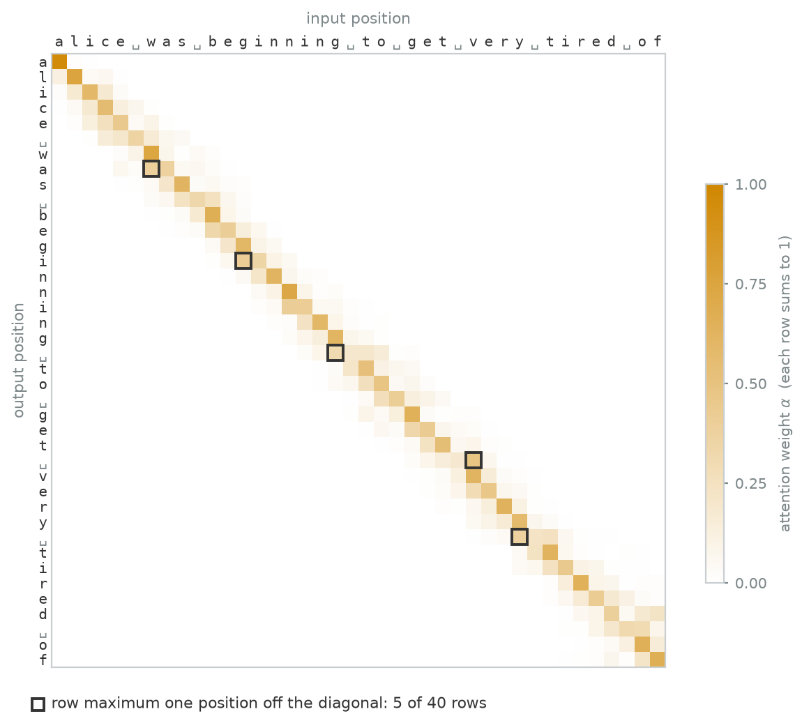
We can inspect which encoder states contribute at each output step. The attention matrix in Figure 8.2 is recorded from a recurrent copy model with attention that we trained on English text, with a state width of 16 (the side quest below compares widths): each row is an output position, each column an input position, and each row sums to one. The 40-character input “alice was beginning to get very tired of” is copied exactly, and the largest weight lies on the matching input position in 35 of the 40 rows, with the other five maxima one character away. Exact copying does not require every row’s maximum to sit on the diagonal, because a recurrent encoder state carries surrounding history and the decoder has a state of its own. Bahdanau et al.’s translation alignments use the same output-by-input view, departing from the diagonal where English and French word order differ [1].
The same score–normalise–combine operation can read a spatial feature grid. We now return to image captioning to see what changes when the source is an image.
8.3 Image captioning with attention
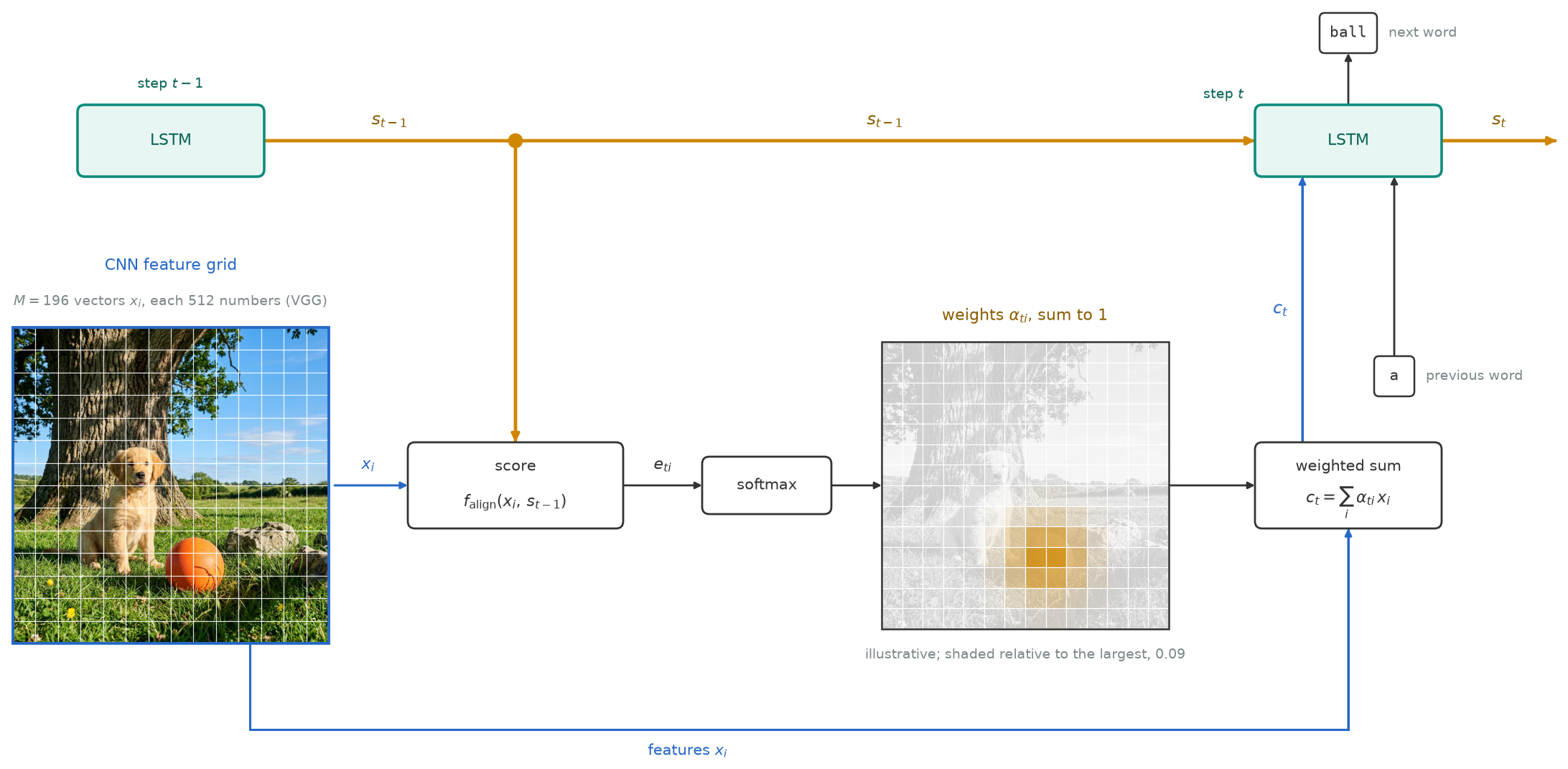
Return to the captioner introduced in the previous chapter. For the scene photograph, a partial caption might end with “a dog is sitting under a tree with a”. Generating “ball” requires information about the small object beside the dog, which may be easier to recover by returning to the image features than by relying on the summary supplied at the beginning.
Show, Attend and Tell retains a spatial CNN feature grid so that the decoder can request a different visual summary at each word [3]. Each location supplies a feature vector. These vectors have receptive fields that extend beyond their grid cells, so a feature at one location need not describe only the pixels directly beneath it.
Let \(x_i\in\mathbb{R}^{d}\) be the feature at image location \(i\) in a grid of \(M\) locations, and \(s_{t-1}\) the decoder’s preceding hidden state. A learned alignment function \(f_{\mathrm{align}}\) assigns a scalar relevance score \(e_{ti}\) to each location. Softmax converts the scores into non-negative weights \(\alpha_{ti}\) that sum to one. Their weighted sum is the visual context \(c_t\), a different quantity from the LSTM cell state that Chapter 7 wrote with the same symbol:
\[ e_{ti}=f_{\mathrm{align}}(x_i,s_{t-1}),\qquad \alpha_{ti}=\frac{\exp(e_{ti})}{\sum_{j=1}^{M}\exp(e_{tj})},\qquad c_t=\sum_{i=1}^{M}\alpha_{ti}x_i. \]
A score measures a learned match; a weight specifies a share of the mixture. The context has the same width as an individual feature vector, and because it is recomputed at every output step, information no longer has to survive exclusively in the decoder’s carried state. The decoder uses this context together with its preceding state and previous word to generate the next word.
The next widget lets us inspect recorded attention from BLIP, a model that generates captions from images [4]. For each generated word, it shows weights over the image features. The request comes from text representations and the information comes from the image: this is called cross-attention. We can follow that exchange without knowing BLIP’s full architecture yet; the rest of the chapter develops the machinery it uses.
Does an object word draw a tighter map than a function word? Commit to an answer, then compare the named objects with “with” in Figure 8.5, reading each word’s peak weight and the number of patches that hold half its attention rather than the brightness of its map.
The recorded caption is “a dog is sitting under a tree with a ball”. Each map is scaled to its own strongest patch, so compare the peak weights and the half-weight counts rather than the brightness: a bright region need not contain most of the attention, and an object word need not have a more concentrated map than a function word.
An attention map shows weights in one computation, not the cause of the final prediction. Jain and Wallace found weak agreement with gradient-based importance and substantially different attention distributions that preserved predictions in their NLP classification and question-answering settings [5]. Wiegreffe and Pinter tested LSTM binary classifiers and argued that conclusions depend on the definition of explanation, the baseline and whether the whole model is considered; their tests included uniform attention, variation across training runs and adversarially trained alternatives [6]. Neither paper establishes what this BLIP caption would do if an image region were removed. A causal claim needs an intervention and a measured change in behaviour, with the intervention itself specified.
Xu et al.’s caption decoder remains recurrent, because it needs its previous state to make the next query. The operation that scores and combines vectors carries no such requirement, and can read spatial features, encoder states or any other collection of vectors.
8.4 Computing attention: queries, keys and values
So far, we have used attention to read encoder states and image features. Here, we name the roles in the computation and express it in a form that handles multiple requests at once. Figure 8.6 provides an overview. Work through the query, key and value stages here, then return to self-attention, masking and multiple heads in the next section.
8.4.1 One query: score, normalise and combine
For each caption word, the decoder makes a request, and the image locations provide information that may answer it. We give the three parts of this computation distinct names: the query describes what is requested, a key helps determine how relevant a source location is, and its value provides the information to combine.
In recurrent captioning, the preceding decoder state (\(s_{t-1}\)) supplies the query, while each image location supplies a key and a value. The query and key determine that location’s score; softmax compares the scores across locations to produce the weights. Each value is multiplied by its weight and added to the context. A key and value refer to the same location, but they need not be the same vector.
Learned projections let a source feature vector provide one representation for matching and another for the information being combined. These are learned linear maps; we do not assign meanings such as “object identity” or “colour” to particular coordinates. A token is one element of a sequence, represented by one vector. In Figure 8.7 each token has a two-dimensional key and a three-dimensional value, displayed as a colour so that the mixture can be seen, and we move the query ourselves. It illustrates the arithmetic without running a learned captioning model.
The captioning model scored each location with a small learned network. Keeping the same score, normalise and combine, but making the scoring a dot product of projected representations, is the whole of the change. For a query \(q\) and keys \(k_i\) of width \(d_k\), scaled dot-product attention computes scores \(e_i=q\cdot k_i/\sqrt{d_k}\), turns them into weights \(\alpha_i=\exp(e_i)/\sum_j\exp(e_j)\) with a softmax, and returns \(o=\sum_i\alpha_i v_i\). The dot product depends on both direction and magnitude, so it is not cosine similarity unless the vectors have also been normalised. Before any subsequent projection, the output is a weighted average of the values, and need not resemble any single one of them.
In Figure 8.7 each token’s key is an arrow and its value is a colour. Point the query between two keys, and say which colour the output will lean towards before reading it off. Then lengthen the query without turning it, and see whether your answer changes. The vector width stays two; this tests score magnitude rather than changing \(d_k\). Finally, switch the scaling off and see whether the same query spreads its weight more or less evenly.
8.4.2 Several queries together
For several queries, place one input vector per row. Let \(X_q\in\mathbb{R}^{N_q\times d_q}\) supply the queries and \(X_s\in\mathbb{R}^{N_s\times d_s}\) supply the keys and values. The learned matrices have shapes \(W_Q\in\mathbb{R}^{d_q\times d_k}\), \(W_K\in\mathbb{R}^{d_s\times d_k}\) and \(W_V\in\mathbb{R}^{d_s\times d_v}\). Thus
\[ Q=X_qW_Q\in\mathbb{R}^{N_q\times d_k},\quad K=X_sW_K\in\mathbb{R}^{N_s\times d_k},\quad V=X_sW_V\in\mathbb{R}^{N_s\times d_v}. \]
The computation is
\[ S=\frac{QK^\top}{\sqrt{d_k}}\in\mathbb{R}^{N_q\times N_s},\qquad A=\operatorname{softmax}_{\mathrm{row}}(S),\qquad O=AV\in\mathbb{R}^{N_q\times d_v}. \]
Row \(t\) of \(A\) holds all the weights used for output \(t\), and its columns index the source vectors, so the row-wise softmax normalises each query’s choices separately. The number of queries and the number of source vectors can differ; what the source must supply is one value for each key. The opening setting of Figure 8.7 is this computation with \(N_q=1\), \(N_s=3\), \(d_k=2\) and \(d_v=3\), with the keys and values given directly rather than projected.
The scale factor addresses how scores tend to grow with key width. A simple case shows why: if \(q\) and \(k\) are both vectors of \(d_k\) ones, then \(q\cdot k=d_k\), so doubling the width doubles the score. Components with mixed signs partly cancel, so the scores of learned vectors need not grow in this way; what matters for softmax is how widely the scores vary, and that can still grow with the width. Under independent, zero-mean, unit-variance component assumptions, a dot product has variance \(d_k\). Its standard deviation — the scale of its fluctuations — is therefore \(\sqrt{d_k}\). Large differences between scores can make softmax concentrate almost all the weight on one key, leaving small gradients for many changes to the scores. Dividing by \(\sqrt{d_k}\) removes this width-dependent variance in that model [7]. That is a rationale, not a guarantee about trained representations.
The spread of \(q\cdot k\) grows with \(d_k\); Figure 8.8 measures what that does to the weights. One draw is noisy, so it also averages the same measurement over many: the red curve is the heaviest weight a softmax puts on one key as the width grows, and the gold curve is the same quantity once \(\sqrt{d_k}\) has been divided out. At a Vaswani head’s width of 64 the unscaled softmax is already spending most of its weight on a single key.
8.5 From cross-attention to self-attention
In cross-attention, queries come from one collection of representations and keys and values from another, as when a text decoder reads image features. Attention gave the recurrent decoder access to its whole input, but left the decoder itself unchanged: it still needed the preceding state before it could process the next word. Self-attention removes that requirement by letting every input position make its own query of the token collection. All queries come from representations already available at the start of the layer, so no state has to be carried through the positions to compute this layer’s outputs.
8.5.1 Self-attention
Let \(X\in\mathbb{R}^{N\times d}\) contain \(N\) token vectors of width \(d\). Self-attention uses the same collection for queries, keys and values:
\[ Q=XW_Q,\qquad K=XW_K,\qquad V=XW_V,\qquad O=\operatorname{softmax}_{\mathrm{row}}\!\left(\frac{QK^\top}{\sqrt{d_k}}\right)V. \]
There is one output row per input token. The matrix products can compute these rows together because none requires another output row from the same layer. This describes how the layer processes available inputs; the causal-mask discussion below explains why generating new tokens still proceeds one step at a time.
Each row of the attention matrix is one token’s query weighing every token. The token making the query also remains among the keys and values, so unmasked self-attention can include the token’s own representation in its output. Without position information or a mask, each token keeps its output when the tokens are reordered, as Figure 8.10 at the end of this section shows.
8.5.2 Multiple heads
One attention head produces one weighted mixture for each query. Several heads let the model form different mixtures in parallel, using different learned representations. Their outputs remain separate until an output projection combines them, so the model can use information from several mixtures in the same update.
Multi-head attention repeats the operation with separate learned projections, so head \(j\) produces \(O_j=\operatorname{Attention}(XW_Q^{(j)},XW_K^{(j)},XW_V^{(j)})\), whose weights and mixture can differ from those of another head. The head outputs are concatenated along their feature coordinates, then an output projection combines them to produce an update of width \(d\):
\[ \operatorname{MHA}(X)=\operatorname{Concat}(O_1,\ldots,O_h)W_O. \]
With \(h\) heads and fixed total width, the usual choice is \(d_k=d_v=d/h\) per head, which requires \(d\) to be divisible by \(h\) and makes the concatenation return width \(d\), with \(W_O\in\mathbb{R}^{d\times d}\). Adding heads therefore divides that width rather than giving every head the full model width. Separate heads provide separate learned mixtures; whether any of them specialises in a relationship a person would name is something to establish by examining the trained model.
8.5.3 Causal and padding masks
A causal mask prevents a query at position \(t\) from using a key at position \(i>t\). Add a mask \(M\) to the scores before softmax, with \(M_{ti}=0\) for \(i\leq t\) and \(M_{ti}=-\infty\) otherwise; since \(\exp(-\infty)=0\), future positions receive no weight.
During next-token training, the full target sequence is known. We shift it to form the inputs: for example, inputs <sos> 4 2 7 predict targets 4 2 7 <eos>. The input at position \(t\) therefore contains the preceding token, and may attend to itself and earlier inputs without seeing its target. The causal mask prevents access to later inputs that would reveal the answer, allowing all training positions to be processed together. During autoregressive generation, each selected token becomes the next input, so it must be generated before the following step can run.
A padding mask separately excludes the filler positions used to batch sequences of unequal lengths. Each active query must retain at least one permitted key, or its softmax is undefined.
In Figure 8.10, switching on the causal mask and then reordering the tokens costs a token its access to everything placed after it — a change in the information permitted, not merely a rearrangement of matrix rows. The mask defines a direction through the sequence without requiring a recurrent state update.
8.5.4 Comparing routes between positions
Compare how information travels between two distant positions in Figure 8.9. A recurrent network passes it along a chain of state updates. A convolution combines nearby positions, so information travels farther as successive layers expand the receptive field. Full self-attention gives each position a direct connection to every position its mask permits [7].
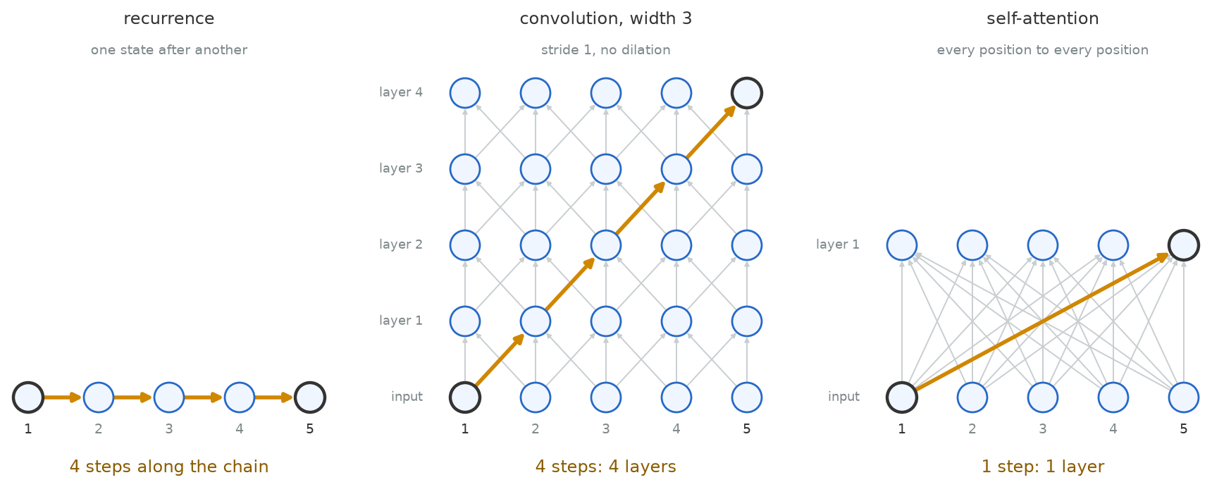
A short path can help information and gradients travel between distant positions, but the model must still learn which relationships are useful. Direct connections also have a cost: full attention compares pairs of positions, so longer sequences create many more comparisons. We return to that cost in the computation and memory section.
Without position information or a mask, reordering the input tokens leaves each token’s output representation unchanged: the output moves with its token. This property is called permutation equivariance. Attention can use the tokens’ content to decide what to combine, but it cannot distinguish different orders of the same collection. A fixed causal mask changes this because moving a token changes which tokens it can use.
Reorder the tokens in Figure 8.10 and follow one of them. Before it moves, predict where its rows in \(X\), \(Q\), \(K\), \(V\) and \(O\) will move, whether the numbers in those rows will change, and what will happen to the attention matrix. Then add position vectors, or switch on the causal mask, and make the same reordering.
8.6 Giving attention a sense of position
Attention needs a way to distinguish the same content appearing at different places. We can supply it by adding a position vector to each token embedding. At position \(p\), the content vector \(e_p\in\mathbb{R}^d\) receives a position vector \(\mathrm{PE}(p)\in\mathbb{R}^d\), giving \(x_p=e_p+\mathrm{PE}(p)\). Both have the same width, so the sum fits the attention layer without changing its shape.
The position vectors stay attached to their locations. Moving a word to another location therefore pairs its content with a different position vector, giving the model information about both what is present and where it occurs. These combined vectors enter the learned query, key and value projections.
One option is to learn a table of position vectors during training. Another is to generate them from a fixed formula. The original transformer’s sinusoidal encoding uses pairs of sine and cosine waves: some coordinates change rapidly with position, while others change slowly. Together they provide a pattern the model can use to distinguish positions and their relationships [7].
For even width \(d\), the formula below gives one sine–cosine pair for each \(i=0,\ldots,d/2-1\). The quantity \(\omega_i\) controls how quickly that pair changes; \(2i\) and \(2i+1\) are its coordinate indices, starting at zero:
\[ \omega_i=10000^{-2i/d},\qquad \mathrm{PE}(p,2i)=\sin(\omega_i p),\qquad \mathrm{PE}(p,2i+1)=\cos(\omega_i p). \]
Binary counting offers a useful comparison. Written in binary, the lowest bit of a position flips at every step, the next bit every two steps and the next every four, so each column changes at half the rate of the one before, and together the columns give every position a distinct code. The sinusoidal encoding is built in a similar way from smooth waves. Its frequencies \(\omega_i\) are geometrically spaced, so the pairs vary at different rates and together carry positional information at several scales, as Figure 8.11 shows. Unlike the bits, whose periods always double, the ratio between successive wavelengths depends on the width \(d\). Each coordinate also varies continuously between \(-1\) and \(1\) rather than jumping between two values, and, as a side quest below shows, a fixed offset acts on each pair in the same way at every position.
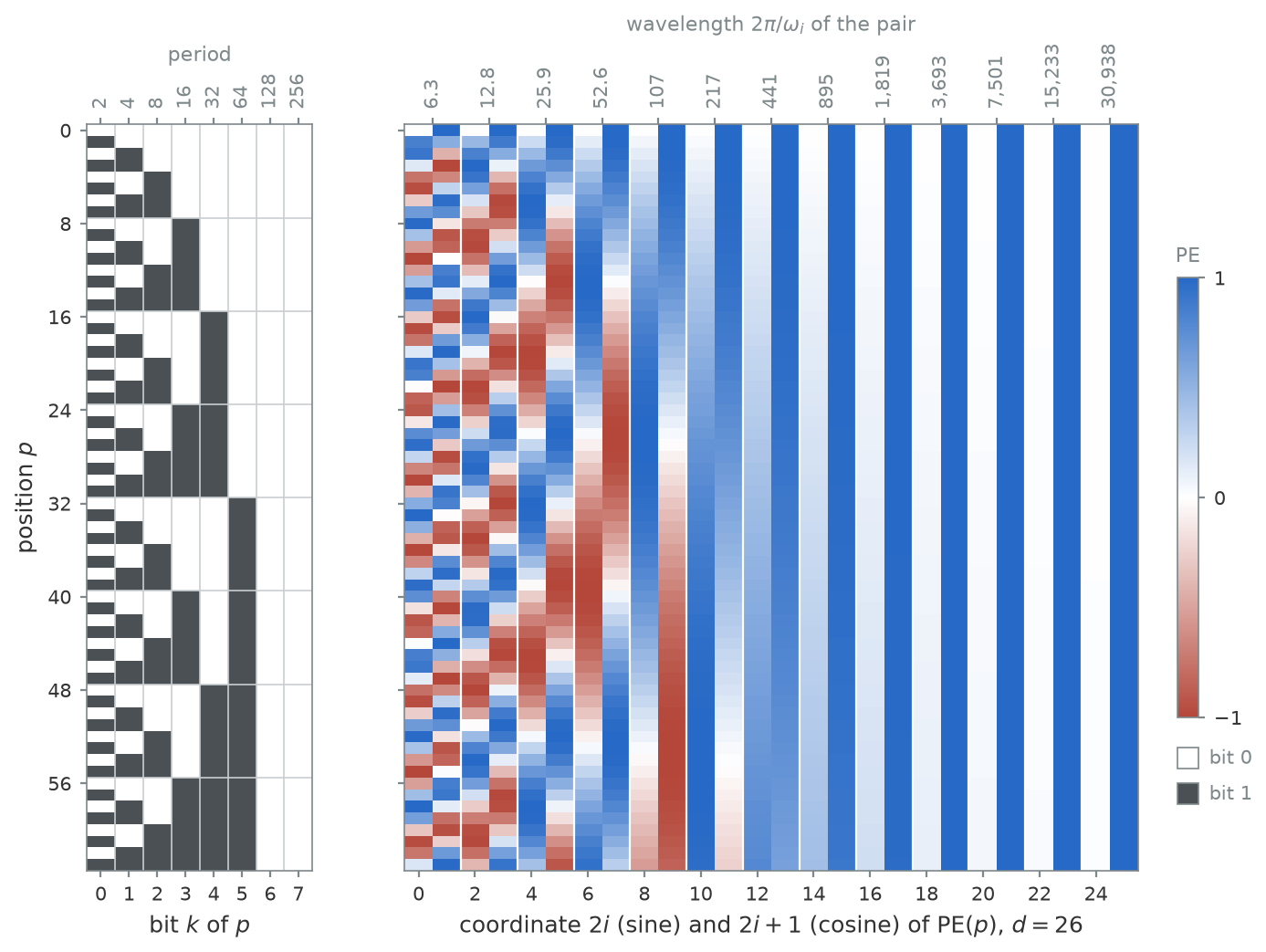
The important construction is a position-dependent vector of the same width as the content, which can be added before attention. A learned table and a fixed formula are both valid choices. A formula can produce codes beyond the positions seen during training, but that alone does not guarantee accurate predictions on longer sequences.
Figure 8.12 shows how the relationship between two position codes changes with their separation; the side quest above explains the pattern. Must their dot product fall at every increase in the gap? Compare pairs at a fixed gap, then widen it and see. Compare the sinusoidal result with the normalised index and the untrained random table. The readout gives the selected pair’s dot product and the range over every pair at the same gap, so the same-gap claim can be checked numerically.
8.7 Assembling the transformer
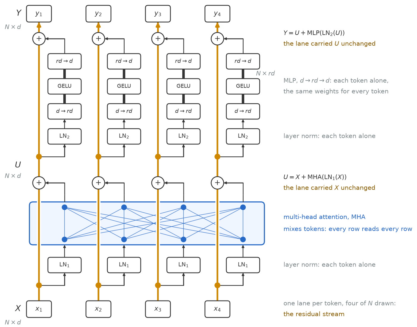
Self-attention lets tokens exchange information. A transformer block follows that exchange with a multilayer perceptron (MLP), a feedforward network that nonlinearly transforms the features each token now holds, applied separately to every token. That division is what the block is built around: attention moves information between tokens, the MLP works on what each token is left holding. Both sit inside residual connections, with layer normalisation controlling the scale of their inputs. The block below uses pre-norm ordering: normalise before each sublayer, then add its output to the saved input. For an input \(X\in\mathbb{R}^{N\times d}\),
\[ U=X+\operatorname{MHA}(\operatorname{LN}_1(X)),\qquad Y=U+\operatorname{MLP}(\operatorname{LN}_2(U)). \]
Both \(U\) and \(Y\) have shape \(N\times d\). The original transformer put the normalisation after each residual addition instead, \(\operatorname{LN}(X+\operatorname{Sublayer}(X))\), which is called post-norm [7]; Figure 8.13 and the widget here use pre-norm throughout, and why that ordering is the common choice now is taken up once the components are in place.
8.7.1 Residual connections
The first residual path saves \(X\) while the attention sublayer computes an update. Adding that update requires the same token count and feature width as \(X\). In the configuration above, concatenating the heads already gives width \(d\); the output projection mixes their contributions while preserving that width. The second path saves \(U\) while the MLP computes another update. A residual addition neither concatenates features nor creates more tokens; it adds corresponding coordinates. What the two paths preserve is a direct route through the block for representations and gradients, which the learned branches modify rather than replace.
8.7.2 Layer normalisation
Layer normalisation standardises the features within one token [8]. For a row \(x\in\mathbb{R}^d\), compute \(\mu=d^{-1}\sum_jx_j\) and \(\sigma^2=d^{-1}\sum_j(x_j-\mu)^2\), then
\[ \operatorname{LN}(x)_j=\gamma_j\frac{x_j-\mu}{\sqrt{\sigma^2+\epsilon}}+\beta_j. \]
The learned scale \(\gamma\) and bias \(\beta\) have width \(d\), and \(\epsilon\) is a small positive constant for numerical stability. Each token has its own mean and variance, while sharing the learned scale and bias with the other tokens in that layer. Like batch normalisation in Section 2.6, this normalises activations and then applies a learned affine transformation; unlike batch normalisation, it estimates nothing across the examples in a minibatch, so it needs no running batch statistics at inference.
8.7.3 The per-token MLP
The MLP expands each token from \(d\) to \(rd\) features, applies a nonlinearity, then contracts it back to \(d\), where \(r\) is the expansion ratio, typically four in the configuration we examine:
\[ \operatorname{MLP}(Z)=\operatorname{GELU}(ZW_1+b_1)W_2+b_2, \qquad W_1\in\mathbb{R}^{d\times rd},\quad W_2\in\mathbb{R}^{rd\times d}. \]
GELU, the Gaussian error linear unit, is a smooth element-wise activation \(\operatorname{GELU}(z)=z\Phi(z)\), where \(\Phi\) is the standard normal cumulative distribution function; the original transformer used ReLU, and GELU is the choice in the ViT-style block examined here. The same MLP weights process every token, and the MLP never reads another token’s row — which is the division the block is built around.
8.7.4 From blocks to models
Because input and output are both \(N\times d\), blocks stack, each with its own learned parameters. Position codes distinguish where content entered, attention combines content across permitted positions, the MLP transforms each row, and the residual paths carry the previous representation around both updates. A pre-norm stack commonly applies a final layer norm after its last block as well. Dropout, which randomly suppresses selected activations during training, can be included in the branches; the diagram omits it to keep the data paths visible.
The arrangement of blocks and masks determines how the model is used:
| Arrangement | Information available to a token | Typical output |
|---|---|---|
| Encoder-only | All unpadded input tokens through self-attention | Contextual input representations for a prediction head |
| Decoder-only | Its own and preceding input positions through causal self-attention | A distribution for the next token |
| Encoder–decoder | Encoder inputs through unmasked self-attention; preceding target context through causal self-attention; encoder outputs through cross-attention | An output sequence conditioned on a separate input |
In the last arrangement a decoder block gains an additional cross-attention sublayer, with queries from the decoder and keys and values from the encoder. This is how captioning connects image representations to a text decoder. The same causal-mask rules govern training and generation.
The block accepts vectors without asking whether they came from words or image regions, and those vectors are constructed from image patches in Chapter 9. First, trace the whole block in Figure 8.14: predict which selected operations can change a token using another token’s content, and check the shapes entering each residual addition.
8.8 Computation and memory
8.8.1 More tokens, more work
Doubling the token count \(N\) in the Explore the cost view of Figure 8.14, with width \(d\) and expansion ratio \(r\) held fixed, moves the two kinds of term differently. The query, key, value and output projections, and both MLP linear layers, perform their work once per token, so their operation counts double. The score product \(QK^\top\) and the weighted-value product \(AV\) involve pairs of positions, so their counts quadruple. These are forward-pass arithmetic counts, not measured training times.
The number of learned parameters stays the same when the input contains more tokens. Each token reuses the same projections and MLP, while attention compares more pairs of positions. Quadratic growth matters increasingly as sequences become longer, but it does not mean that the attention products dominate every configuration. Arithmetic counts also differ from measured runtime: implementations and hardware affect how quickly the operations run.
8.8.2 What training keeps in memory
Memory during training is harder to predict than either count. It includes the parameters, their gradients, the optimiser’s state, the activations saved for backpropagation, input tensors and temporary workspace, and an allocator also reserves blocks that may not all contain live tensors. Allocated memory counts storage currently used by tensors, while reserved memory includes space held by the allocator for reuse; the peak of each is measured over a run, and the two peaks need not occur at the same instant. The implementation matters as well: a straightforward attention implementation can store an \(N\times N\) weight matrix per head, whereas implementations that avoid materialising the full matrix can have different memory use despite computing the same attention operation.
8.8.3 Mixed precision and gradient accumulation
Mixed precision uses different numerical formats within one computation. Selected operations and saved intermediates can use a lower-precision format while parameters and optimiser state remain in a higher-precision format. This can reduce memory use, but does not imply that the whole training footprint halves. The measured example in Chapter 9 shows which parts change.
A micro-batch is the set of examples processed in one forward and backward pass. Gradient accumulation adds gradients from several micro-batches before making one optimiser update. With equally sized micro-batches and losses scaled to average across them, the effective batch is the micro-batch size times the number of accumulation steps. Four passes of 32 examples therefore supply an effective batch of 128, while the saved activations need only cover one pass at a time. The gradients persist between passes; the earlier computation graphs need not.
Mixed precision changes the numerical formats used within a pass. Accumulation changes how many passes contribute to an update. They can be used together, and neither removes the need to measure memory for the actual training configuration.
The transformer block is now complete: position information distinguishes locations, attention mixes information across permitted tokens, and the MLP transforms each token’s features. In Chapter 9, image patches supply those tokens. That chapter also contains the detailed ViT cost calculations, recorded GPU measurements and memory-budget widget beside its fine-tuning practical.
Exercises
- What changes when the context changes? Compare the copying encoder–decoder from Chapter 7 with one that uses attention. What information can the decoder access at each output step? Each context vector still has a fixed width: explain why the input no longer has to be represented only by the encoder’s final state.
- Score, normalise and combine. A query assigns equal scores to three source positions whose value vectors are \((1,0)\), \((0,2)\) and \((2,1)\). Compute the attention weights and output vector. Now use weights \((0.6,0.3,0.1)\) and compute the new output. What information do the weights describe, and why need the output match none of the individual values?
- Following the shapes. Two queries attend to three source vectors. Queries and keys have width four; values have width two. Give the shapes of \(Q\), \(K\), \(V\), \(QK^\top\), \(A\) and \(AV\). Along which axis is softmax applied? Explain why there must be one value per key, but not necessarily one key per query.
- Which information is available? Draw the allowed attention entries for four positions under unmasked self-attention and under causal self-attention. With inputs
<sos> 4 2 7and targets4 2 7 <eos>, explain why a position may attend to its own input without seeing its answer. Why can these training positions be processed together while generation proceeds one token at a time? How does a padding mask serve a different purpose? - Content and position. Consider unmasked self-attention with no position information. If the input tokens are reordered, what happens to their corresponding outputs? Explain how adding position vectors changes the experiment when content moves but the position vectors stay attached to their locations. Does a sinusoidal code being defined beyond the training range guarantee good predictions there?
- Building a block. Sketch a pre-norm transformer block with both residual paths. Mark which operations combine information from different tokens and which process each token separately. Why must the attention output projection and the MLP return the original feature width? Explain what several heads add beyond a single weighted mixture.
- More tokens or a larger batch? With feature width fixed, predict what doubles and what quadruples when token count doubles: projection work, attention score entries, MLP work and parameter count. Then explain how accumulating gradients over four micro-batches changes the effective batch and the activations that must be kept at once. How does mixed precision address a different part of the memory problem?
- Testing the new route to the input. Design a comparison between a fixed-context digit reader and an attention-based reader. State what you would keep the same, how you would test lengths seen and unseen during training, and what exact-string accuracy and character error rate would each reveal. If an attention map concentrates on a digit, what does that show about the computation, and what further evidence would you need to claim that region caused the prediction?
Lab 8
Lab 8: adding attention to the Lab 7 digit reader. A bidirectional GRU keeps a state for every column of the strip; a fixed-context reader and an attention reader share it, and are compared by exact-string accuracy and character error rate within and beyond the training lengths, with the attention maps of correct readings and failures.

Further reading
- Bahdanau et al. [1] — learning to align and combine encoder states for translation.
- Xu et al. [3] — generating captions with attention over spatial image features.
- Vaswani et al. [7] — the transformer’s attention, positional encoding and encoder–decoder blocks.
- Li et al. [4] — the vision–language model used for the recorded caption-attention example.
- Rush [10] — an annotated PyTorch implementation of the transformer, with layer normalisation before each sublayer as in this chapter’s block, and the paper’s text alongside the code.