6  Segmentation

NoteLearning objectives

• Distinguish semantic, instance, and panoptic segmentation
• Interpret segmentation metrics and explain why pixel accuracy can hide failure
• Explain how fully convolutional networks share computation across spatial predictions
• Build and train a U-Net and explain why skip connections matter
• Describe atrous convolution and ASPP (DeepLab) at a conceptual level; explain Mask R-CNN’s RoIAlign
• Explain how output channels, loss and training pairs adapt a U-Net to different image-to-image tasks

Skills ladder. Checkpointing and resuming; log checkpoints as W&B artefacts. Chapter 14’s lab resumes from this pattern.

Detection returns a rectangle, which gives only a coarse answer: the axis-aligned box around a dog standing on grass contains mostly grass. Segmentation provides an answer at full resolution, describing objects and regions pixel by pixel.

Three different tasks go by that name, each producing a different output: a class map, a set of object masks, or a partition of the image into labelled segments. The metrics come first because they define what each of the three benchmarks measures.

6.1 Three segmentation tasks

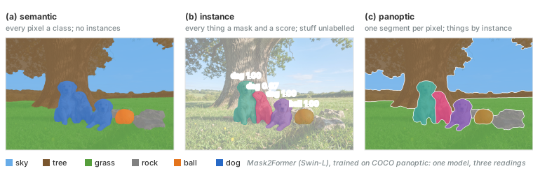
Semantic segmentation assigns a class to every pixel, producing a single label map with no concept of individual objects. Two dogs side by side both receive the label “dog,” with no way to tell them apart. If they do not touch, you could count the connected components afterwards, but that adds a guess on top of the output—and fails as soon as the dogs overlap.

Instance segmentation assigns a mask to each object. Two dogs are represented by two masks, each with its own class and score. Predicted masks may overlap, but ordinary instance segmentation aims to outline each object’s visible region, not reconstruct its hidden parts. Only things receive a mask, so the grass and the sky, and with them most of the frame, remain unlabelled. Mask R-CNN adds a mask to each detected object, as Section 6.6 explains.

NoteThings and stuff

A thing is a countable object with a definite extent: a dog, a ball, a person, a car. It makes sense to ask how many there are, so we can give each one its own identity and a class.

Stuff is an amorphous region of material or texture with no natural boundary between one piece and the next: grass, sky, road, water. Asking how many grasses there are has no answer, so stuff is labelled by class alone.

The three tasks differ in how they treat the two. Semantic segmentation labels things and stuff alike but does not distinguish individual objects. Instance segmentation labels things only, each separately. Panoptic segmentation labels both, and separates the things.

Panoptic segmentation [1] asks for both at once: every pixel is assigned exactly one (class, instance) pair, and segments may not overlap. Stuff pixels receive a class, but no instance identifier, and thing pixels receive both. One output, no gaps, no overlaps.

Figure 6.1: One Mask2Former model trained on COCO panoptic segmentation produces three outputs for one photograph. (a) Semantic segmentation assigns every pixel a class; the three dogs share one label. (b) Instance segmentation gives each dog a separate mask and score, leaving stuff unlabelled. (c) Panoptic segmentation labels every pixel and distinguishes the individual dogs. COCO treats rock as stuff, so the rocks form one segment. Our own runs (figures/runs/ch06_runs.py).

The output determines what we need to measure: pixel labels, individual object masks, or a complete partition of the image.

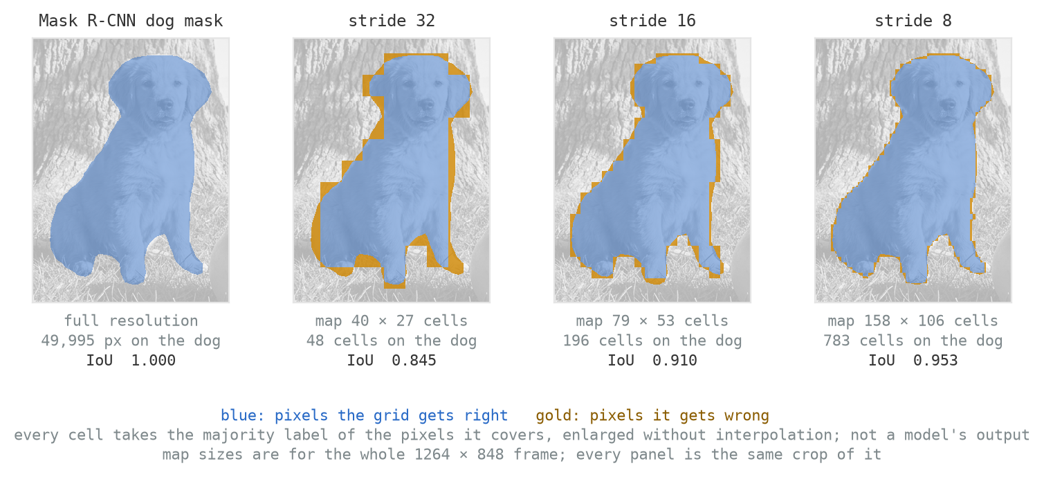
Pixel accuracy is the fraction of pixels assigned the correct label. Although it is often the first metric reported, it can be misleading when one class dominates an image—a common issue in segmentation, where much of the image may be background. Take Mask R-CNN’s mask of the dog in our photograph as the reference. It covers 49,995 of the image’s \(1264 \times 848 = 1{,}071{,}872\) pixels, or 4.7% of the frame. A model that labels every pixel as background and returns no mask would therefore achieve 95.3% pixel accuracy. Reporting such a high score may lead readers to believe the model performs well, even though it has learned nothing.

Intersection over union (IoU) is calculated separately for each class, so true negatives from the background do not inflate the object class’s score. It uses the same formula as the box metric in Section 4.1, applied to sets of pixels: for class \(c\), IoU is the intersection of the pixels predicted as \(c\) and the pixels that are actually \(c\), divided by their union. Mean IoU (mIoU) averages these scores across classes. An all-background model scores 0 IoU for dog because it finds none of the dog pixels, and 0.953 for background, giving a mean IoU of 0.477. The difference from pixel accuracy lies in the true negatives. Pixel accuracy counted every background pixel the model correctly left out of the dog; the dog’s IoU counts only pixels that are dog or were called dog, so those correctly rejected pixels contribute nothing to either its numerator or its denominator. With no dog pixels found, the intersection is empty, and the dog’s IoU is zero. mIoU is the headline metric on semantic segmentation benchmarks.

ImportantIoU, mean IoU and Dice

For class \(c\), let \(P_c\) be the set of pixels the model assigns to \(c\) and \(G_c\) the set of pixels whose ground-truth label is \(c\). Then

\[ \mathrm{IoU}_c = \frac{|P_c \cap G_c|}{|P_c \cup G_c|}, \qquad \mathrm{mIoU} = \frac{1}{C} \sum_{c=1}^{C} \mathrm{IoU}_c, \]

where \(C\) is the number of classes. On the benchmarks, each class’s intersection and union are summed over the whole dataset before the division, rather than averaged image by image.

The Dice coefficient (Sørensen–Dice) counts the intersection twice and divides by the sum of the two areas rather than their union:

\[ \mathrm{Dice}_c = \frac{2\,|P_c \cap G_c|}{|P_c| + |G_c|} = \frac{2\,\mathrm{IoU}_c}{1 + \mathrm{IoU}_c}. \]

Figure 6.2: These set diagrams show IoU and Dice for the pixels predicted as a class, P, and the ground-truth pixels of that class, G. Solid regions are the areas each formula counts. IoU divides the overlap by the union; Dice divides twice the overlap by the sum of the two areas.

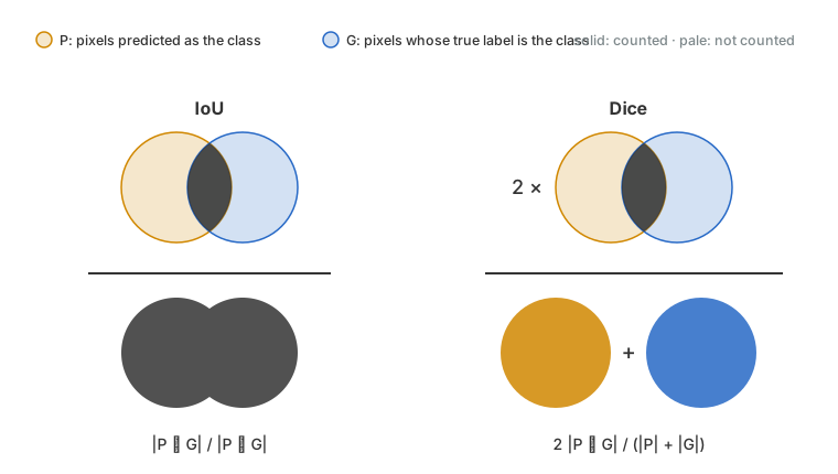
In the Dice denominator the overlap is counted twice, once inside each area, which is why the numerator counts it twice as well: a perfect prediction still scores exactly 1.

The second form follows from \(|P_c| + |G_c| = |P_c \cup G_c| + |P_c \cap G_c|\). In pixel counts, IoU is \(TP/(TP+FP+FN)\) and Dice is \(2TP/(2TP+FP+FN)\), the \(F_1\) score over pixels; neither contains the true negatives, which is why neither is inflated by the background.

Dice increases with IoU, so the two rank predictions for a single mask identically. For any prediction that overlaps the target only partly, Dice gives the higher value; the two agree at no overlap and at perfect overlap. Averaging over images or classes can nevertheless rank two models differently, because the conversion is nonlinear.

Dice is widely used in medical image segmentation. Replacing hard pixel assignments with predicted probabilities gives a differentiable soft Dice score, commonly used as a loss by subtracting it from one. Foreground Dice emphasises overlap without rewarding correctly rejected background pixels. It is not immune to background errors: foreground probabilities assigned to background pixels still contribute to its denominator.

TipDice or IoU?

Use the metric reported by the benchmark or baseline: typically mean IoU for scene parsing and Dice for medical image segmentation. Dice and IoU have different scales, so their values should not be compared as if they were interchangeable.

Figure 6.3: The curve relates Dice to IoU for the same prediction: Dice = 2·IoU/(1 + IoU). The two agree at 0 and 1. Between these endpoints Dice is higher, with a maximum gap of about 0.17 at IoU ≈ 0.41.

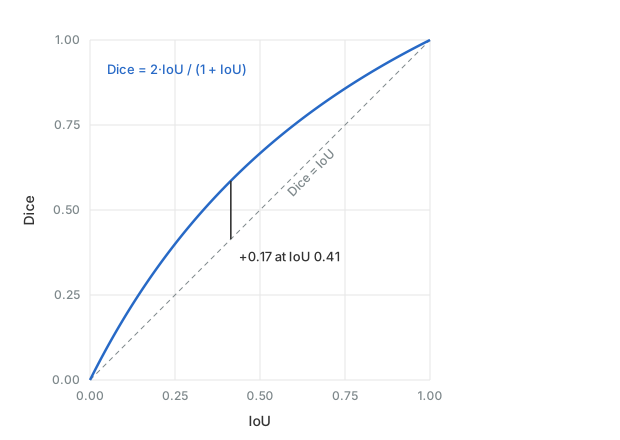
The curve lies above the diagonal everywhere between the two ends, so the same prediction always reads higher as Dice; the gap is widest in the lower middle of the range and closes at both ends.

Mask average precision (mask AP) evaluates instance segmentation using the same confidence-ranked predictions and matching procedure as detection AP (Section 4.1), but measures overlap between masks instead of boxes. A prediction must have the correct class and sufficient mask IoU with an as-yet unmatched ground-truth instance. Missed objects, duplicate detections and inaccurate masks therefore affect the score. COCO-style mask AP averages across classes and several IoU thresholds.

Panoptic quality [1] evaluates the third task by measuring both whether the correct segments were found and how accurately they were outlined. A predicted segment matches a ground-truth segment if they have the same class and their IoU is strictly greater than 0.5. Because panoptic segments do not overlap, a threshold above 0.5 ensures that each ground-truth segment can match at most one prediction. This yields true positives, unmatched predictions (false positives), and unmatched ground-truth segments (false negatives), from which PQ is calculated.

ImportantPanoptic quality

For one class, with \(TP\) the set of matched (prediction, ground truth) pairs,

\[ \mathrm{PQ} = \frac{\sum_{(p,g) \in TP} \mathrm{IoU}(p, g)}{|TP| + \tfrac{1}{2}|FP| + \tfrac{1}{2}|FN|}, \]

and the final score averages PQ over classes. When there is at least one match, multiplying the expression by \(|TP|/|TP|\) splits it into two factors:

\[ \mathrm{PQ} = \underbrace{\frac{\sum_{(p,g) \in TP} \mathrm{IoU}(p, g)}{|TP|}}_{\text{segmentation quality, SQ}} \times \underbrace{\frac{|TP|}{|TP| + \tfrac{1}{2}|FP| + \tfrac{1}{2}|FN|}}_{\text{recognition quality, RQ}}. \]

SQ is the average IoU of the matched segments, so it measures how well they are outlined. RQ is the \(F_1\) score over segments, so it measures recognition: it falls with every missed segment and with every false one. A model that outlines beautifully but misses half the objects and a model that finds everything and outlines it roughly can reach the same PQ, and the factorisation says which is which [1].

Figure 6.4 runs the pixel-accuracy argument on the real mask.

Figure 6.4: This widget compares pixel accuracy and IoU as a reference mask is degraded. The reference is Mask R-CNN’s dog mask, which covers 4.7% of the frame; the slider erodes, dilates or shifts a copy, and the dashed line marks the score of an all-background prediction. Before moving the slider, predict both metrics for an empty mask. Then erode by 20 pixels: accuracy changes little, while IoU falls substantially. Numbers computed in figures/verify_numbers.py.

6.2 Classifying one window at a time

The most direct way to label every pixel in an image is to use a classifier. Crop a small window centred on a pixel, classify it, and assign the resulting label to the centre pixel. Move the window one pixel and repeat until every pixel has served as the centre. The window provides context that an isolated pixel lacks: a patch of brown fur may be ambiguous, but one that also contains an ear and an eye is not. Cireşan et al. used exactly this approach to segment neuronal membranes in electron-microscopy images, winning the ISBI 2012 challenge [2]. Their sliding-window network held the best result on that benchmark until U-Net (Section 6.4) improved on it, mainly by making fewer topological mistakes: fewer broken or merged membranes.

Figure 6.5: This widget compares classifying one window per position with processing the image in one pass. An ImageNet ResNet-50 classifies a window centred on every 16th pixel, and the right panel counts how many windows read each pixel. Before switching to one pass, predict that count. In one pass, an FCN computes the features once and neighbouring outputs share them.

The problem is computational cost. Our photograph contains over a million pixels, so labelling it this way requires over a million forward passes—one per window. Neighbouring windows share almost all their pixels. Because a convolution’s output at each position depends only on the surrounding pixels, the early layers repeatedly compute nearly identical features across overlapping windows. Much of this work is redundant.

R-CNN (Section 4.2) faced the same inefficiency with region proposals: roughly two thousand overlapping crops per image, each requiring a separate forward pass. Fast R-CNN (Section 4.3) eliminated this waste by running the backbone once over the entire image and extracting each region’s features from the resulting shared feature map. The same idea applies here: compute features for the whole image in a single forward pass, then use the shared feature map to predict the pixel labels.

6.3 Fully convolutional networks

A convolutional layer already processes an image in the way we need: it applies the same learned filters at every spatial position, producing a map of features. The obstacle is the classifier at the end. In a network such as VGG-16, the feature map is flattened and passed through dense layers to produce one vector of class scores. These layers expect a fixed number of inputs, so we cannot simply feed the network a larger image and obtain a larger map of predictions.

Section 2.5 showed how to reinterpret a dense layer as a convolution. If the dense layer reads an entire feature volume, the equivalent convolution has a kernel that spans that volume’s height and width and reads all its channels. On the original feature volume, it produces the same output using the same weights.

For example, VGG-16’s first dense layer reads a feature map with \(7 \times 7\) spatial positions. Rewriting it as a \(7 \times 7\) convolution, with no padding and with each filter reading all input channels, produces the same feature vector at a single output position. On a larger feature map, the same filters slide across several positions, producing a feature vector at each one. The remaining dense layers mix the values within each vector without reading neighbouring positions, so they become \(1 \times 1\) convolutions. What was one classifier output is now a spatial grid of outputs, all computed with the same learned weights.

Figure 6.6: An FCN reads the whole image and returns one score map per class. The convolutional stages reduce each spatial dimension by a factor of 32, and a final 1 × 1 convolution gives one channel per class. Argmax across the channels selects each position’s label. Four of the 21 Pascal VOC maps are shown, from FCN-ResNet50 on our photograph; that network predicts at stride 8, so its probabilities are averaged over 32 × 32 blocks to match the diagram.

Figure 6.7: The FCN’s output forms a volume with one score map per class. Hover over a slice or class to see its map and where argmax selects that class. The widget opens on a hand-built six-class illustration; a switch shows real 21-class FCN-ResNet50 scores. Before switching, predict how FCN-ResNet50 labels sky, tree and grass when these classes are absent from its vocabulary.

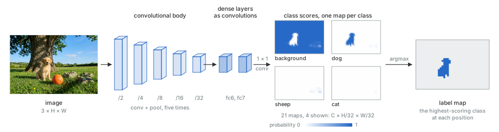
Long, Shelhamer, and Darrell used this conversion to adapt pretrained classification networks for semantic segmentation [3]. They replaced the original classification output with a \(1 \times 1\) convolution that predicts the segmentation classes. The converted layers retain their pretrained weights; the new output layer was trained from scratch, and the network was fine-tuned for segmentation. The result was a fully convolutional network (FCN): a whole image enters the network, and a spatial map of class scores is produced with a single forward pass.

Each output position uses the same learned weights, and overlapping receptive fields share the computation of the earlier layers. Making the network fully convolutional therefore solves the repeated-computation problem. It does not solve the resolution problem: pooling and strided layers still downsample the image, so the predictions lie on a coarse grid. Upsampling restores the output dimensions; skip connections bring in finer information to improve localisation.

VGG-16’s pooling stages give an output stride of 32: neighbouring positions in the score map are 32 pixels apart in the input. Their receptive fields are much larger and overlap, but the network produces scores only at these widely spaced positions. This limits how precisely the coarse map can represent an object’s boundary.

FCN-32s upsamples the coarse class-score maps using a transposed convolution (Section 2.4), with padding and cropping used to align the output with the input image. In the original implementation, this final upsampling layer is fixed to perform bilinear interpolation [3]. Each class’s scores are interpolated separately; selecting the highest-scoring class at each pixel then produces the label map. The output has the required spatial dimensions, but interpolation cannot recover boundary detail absent from the coarse scores.

Figure 6.8: Upsampling converts coarse scores into a label at every pixel. The left panel shows FCN-ResNet50’s dog scores averaged over 32 × 32 blocks, one value per block. Before trying both methods, predict how enlarging the labels differs from interpolating the scores and then thresholding. The right panel compares the resulting mask with Mask R-CNN’s outline. Interpolation gives smoother boundaries, but neither method recovers detail absent from the coarse scores.

Training uses the upsampled scores and a ground-truth label map. At each labelled pixel, a softmax over classes and the cross-entropy loss of Section 2.6 measure the prediction error. The losses are summed over the image, and gradients pass through the upsampling layer to train the network.

Figure 6.9: The left panel follows one pixel on the dog’s boundary across all six class maps. A softmax converts its scores to probabilities, 0.60 for dog, and cross-entropy against the ground-truth label gives −log 0.60 = 0.51. The right panel shows the loss at every pixel, largest along the boundaries in this example. Training sums these losses. Scores from the illustration of Figure 6.7.

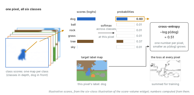
The foreground/background imbalance discussed in Section 6.1 also affects this loss. When most labelled pixels are background, most loss terms concern background. Their combined contribution can outweigh the foreground terms, depending on the prediction errors. This is the same imbalance that motivated focal loss in Section 5.2.

FCN-16s improves localisation by combining the coarse prediction with predictions from an earlier, finer feature map. A \(1 \times 1\) convolution turns that earlier map into class scores. The coarse score maps are upsampled to the same resolution, aligned with the finer maps, and added to them, class by class. This connection from an earlier layer to the output is a skip connection. The combined scores are then upsampled to the input resolution.

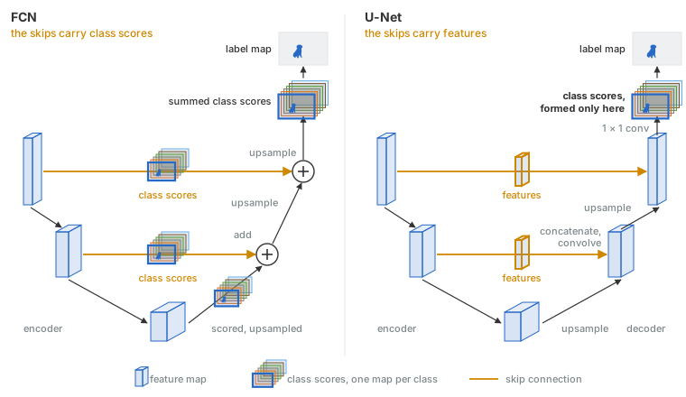
FCN-8s repeats this process with another, still finer feature map. The names refer to the stride of the finest score map used before the final upsampling. The earlier layers retain more spatial detail, while the deeper layers provide richer information about object identity. Combining their predictions improves localisation [3]. Each skip is converted to class scores before addition: FCN combines predictions from different depths. U-Net, in Section 6.4, instead passes feature maps to a decoder that learns how to combine them.

Figure 6.10: FCN-16s adds class scores from two depths. Scores from the deep, coarse features are upsampled by 2; the earlier, finer features arrive along the gold skip and are converted to scores by their own 1 × 1 convolution. The score maps are added class by class, then upsampled to the input resolution. The dog maps are block-averaged versions of a real mask, to show how much detail the finer grid retains.

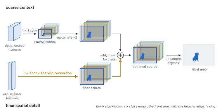
Figure 6.11 illustrates how a coarser grid loses detail around narrow structures and boundaries.

Figure 6.11: The same dog mask is averaged within each cell of progressively finer grids, thresholded at half coverage and enlarged. The coarse grids lose detail in the legs and ears. These are reconstructions from the mask, not model predictions.

6.4 U-Net

FCN combines class predictions from different depths to improve localisation. U-Net instead passes earlier feature maps into a decoder that progressively rebuilds spatial resolution [4]. This gives the decoder access to features that describe both what is present and where its boundaries lie.

Figure 6.12: FCN and U-Net pass different information through their skip connections. In FCN, each skip carries class scores, and the upward path adds score maps. In U-Net, each skip carries encoder features, which a decoder stage concatenates with the upsampled features before convolving them. Class scores appear only at the output.

The encoder follows the familiar classification-network pattern: convolutions extract features, and pooling reduces their spatial resolution. Deeper features draw on larger regions of the input, providing context that helps distinguish objects and materials. However, repeated downsampling makes fine spatial detail harder to retain.

Figure 6.13: Receptive fields grow through U-Net’s encoder. The left panel marks one position at each level, each level in its own colour; the right panel shows the receptive field of each in the same colour, to scale on a 572 × 572 tile: 5, 14, 32, 68 and 140 pixels across. Deeper levels have lower spatial resolution but draw on more context.

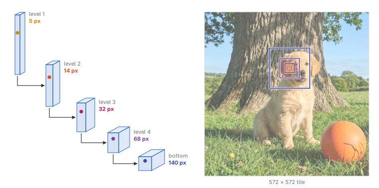
The decoder reverses the direction of this progression. At each stage, it upsamples its feature map and applies convolutions to refine it. Upsampling alone cannot restore information lost during downsampling, so a skip connection brings in the encoder’s features from the corresponding spatial scale. The decoder combines these finer features with the context carried up from deeper layers.

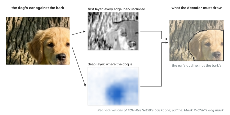
Consider the boundary between a dog’s ear and the tree bark behind it. Deep features may establish that this region belongs to a dog, while earlier features retain more precise information about the local edges. The skip connection gives the decoder access to that information without requiring it to survive every downsampling stage. The decoder still has to learn which edges belong to the object.

Figure 6.14: Early and deep features carry different information about the boundary. An early layer responds to the bark’s edges as strongly as to the ear’s. A deep layer marks where the dog is, but only coarsely. The outline on the right follows the ear’s edge and ignores the bark’s, which takes both. Real FCN-ResNet50 activations on our photograph, computed in figures/ch06_computed.py.

U-Net joins the two feature maps by concatenating them along the channel dimension. Their spatial positions must align, but their channels are placed alongside one another. The following convolution learns how to combine them. Addition would merge corresponding channel values immediately; concatenation keeps the two sources separately available to the next layer.

Figure 6.15: At one decoder stage, the upsampled deeper features and the encoder features from the gold skip are concatenated along the channel dimension. The next convolution receives both sources separately and learns how to combine them. The inset shows addition, which would instead merge corresponding channels before this convolution.

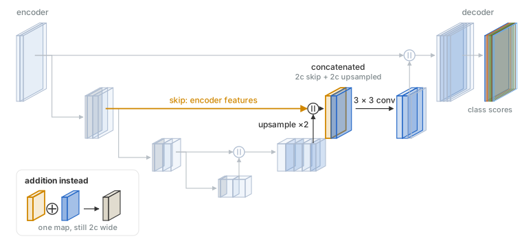
This process repeats at progressively finer resolutions. A final \(1 \times 1\) convolution maps the resulting features to class scores, and training uses the same per-pixel loss described for FCN. Drawn with the encoder descending, the decoder ascending and skip connections crossing between them, the architecture forms the U that gives it its name.

For binary segmentation, a single output channel with a sigmoid and binary cross-entropy can replace the multiclass softmax formulation. That channel predicts foreground membership, with background represented by its complement; this provides a suitable setup for the binary segmentation task in Lab 6.

Figure 6.16 shows how the encoder, decoder and skip connections fit together.

Figure 6.16: This widget traces the feature maps through U-Net’s encoder and decoder. Hover over a decoder stage to inspect the features it concatenates. Before switching to same padding, predict what happens to the crops on the skip connections.

NotePadding and image borders

The original U-Net used valid convolutions, without padding, so every convolution trims the map and the output is smaller than the input: a 572 × 572 tile gives a 388 × 388 prediction. Encoder features are therefore cropped to match their decoder partners at each skip, which is what the crop-and-copy arrows on the familiar diagram show. To cover a large image, the authors ran overlapping tiles and mirrored the image at its borders to supply the missing context. Many implementations use same padding to avoid shrinkage within the convolutional blocks. With input dimensions that fit the downsampling and upsampling stages, this allows matching skip sizes and an output the same size as the input. Other input sizes may still require padding, cropping or explicit size adjustments. The padding switch in Figure 6.16 shows the difference.

6.4.1 Training with limited labelled data

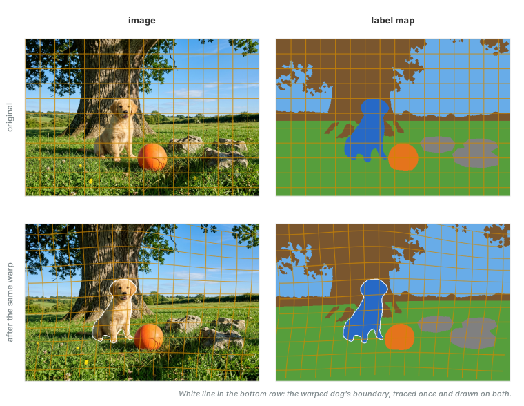
U-Net was developed for biomedical segmentation, where labelled images are scarce. Its first benchmark provided only 30 annotated electron-microscopy images. The authors relied heavily on data augmentation, especially elastic deformations: smooth random warps applied identically to each image and its label map, giving the network new shapes without new annotations [4].

Figure 6.17: U-Net used elastic deformation for data augmentation. One smooth random warp is applied to both the photograph and its label map, so the white boundary traced from the labels stays aligned with the warped dog. One annotation can therefore supply many training examples.

For cell images the authors also weighted the loss, giving extra weight to the thin background gaps between touching cells, so that filling a gap, and so merging two cells into one, costs more than other mistakes. The original weight map combines class balancing with this extra emphasis on boundaries between instances. Weighting the gaps encourages separation without guaranteeing it.

NoteUpsampling and checkerboard artefacts

Transposed convolutions can produce checkerboard patterns when their output patches overlap unevenly, as Figure 2.16 counts and Figure 2.17 shows in a generator’s output. This happens when the kernel size is not divisible by the stride. The original U-Net’s up-convolutions avoid this specific mechanism, although even overlap does not guarantee artefact-free results. One alternative is to resize the feature map first, then apply an ordinary convolution [5].

The encoder serves as the network’s feature-extracting backbone (Section 3.4). U-Net’s own was trained from scratch in 2015, but modern implementations often initialise the encoder with weights from a pretrained classification network, attach a new decoder, and fine-tune some or all of the combined model.

6.5 DeepLab ideas in brief

FCN and U-Net recover spatial resolution after the encoder has reduced it. DeepLab explores a complementary approach: reduce the amount of downsampling in the later backbone stages, so the network retains finer feature maps. The challenge is to do this without losing the broad context needed to recognise objects.

Pooling and strided convolutions reduce the number of spatial positions at which features are computed. Relative to the original image, these positions become more widely spaced: the network has a feature vector for each location on a coarse grid, rather than for every input pixel. A convolution on this grid covers a larger region of the original image, but evaluates features at fewer locations. Upsampling afterwards fills the spaces between those locations without computing new features from the image there.

Atrous convolution, also called dilated convolution (Section 2.4), separates these two effects. It spaces the kernel’s sampling points farther apart, increasing its receptive field without increasing the number of weights. Crucially, the kernel can still move across the feature map one position at a time. Each individual computation samples widely spaced locations, but the output is evaluated densely.

DeepLab uses this to remove some of the later downsampling while increasing dilation in the convolutions that follow. The network retains a finer grid of feature vectors, and each vector still draws on a broad region of the image. It therefore combines the context needed for recognition with denser spatial information for localisation [6]. Figure 6.18 compares the two routes.

Figure 6.18: Atrous convolution uses widely spaced taps but evaluates them at every position. (a) Downsampling, convolving and upsampling computes every second output and fills in the hatched ones. (b) An atrous convolution at rate 2 reads the same footprint at every position: the gold taps of one output and, in grey, those of its neighbour one cell along.

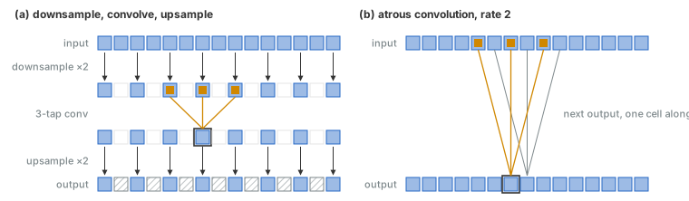
On the photograph the two routes turn out to be the same calculation. Convolving the half-size copy reads exactly the pixels that the rate-2 kernel reads on the full image, with the same weights, so wherever the downsampled route produces an output, it agrees with the atrous one, except near the image borders, where the two routes pad differently. The atrous convolution also computes the outputs in between, which the downsampled route can only fill in.

Figure 6.19: This widget applies one 7 × 7 edge kernel to the photograph by both routes: (a) to a copy that keeps every second row and column, its outputs placed back on the full grid, and (b) at rate 2 to the full image. Point at a pixel of either output to see the input pixels each route reads and both values there. Before pointing at an odd pixel, predict what (a) has there, and which input pixels (b) reads. Then switch (a)’s missing pixels to nearest or bilinear and see where the filled-in values differ from (b)’s.

The trade-off is captured by output stride: the spacing between neighbouring feature-map positions measured in input pixels. A smaller output stride gives a finer grid, which helps localisation, but requires more memory and computation. Halving the stride doubles the map’s height and width, so later layers process four times as many positions. Dilation does not add kernel weights, but retaining larger, densely computed feature maps still costs more.

Objects appear at different sizes, and the context needed to recognise them varies. A small neighbourhood may reveal an edge or texture; a larger one may reveal the surrounding object or scene. DeepLab combines these views using atrous spatial pyramid pooling (ASPP).

ASPP sends the same feature map through parallel convolution branches with different dilation rates. Their outputs retain the same spatial dimensions but draw on different amounts of surrounding context. The branches are concatenated along the channel dimension, and a further convolution learns how to combine them. Like the Inception blocks of Section 3.1, ASPP combines parallel views at different scales; here, dilation controls the sampling footprint.

Figure 6.20: Atrous spatial pyramid pooling sends one feature map through five parallel branches: a 1 × 1 convolution, three 3 × 3 convolutions at increasing dilation rates, and an image-level branch that uses global average pooling. Their outputs are concatenated and combined by a 1 × 1 convolution. The inset shows how outer taps can fall on padding at large dilation rates.

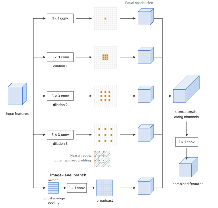
Increasing dilation indefinitely does not provide reliable whole-image context. On a finite feature map, widely spaced sampling positions can fall outside the map and read padding. DeepLabv3 therefore adds an image-level branch: global average pooling summarises each channel across the whole map, a convolution transforms that summary, and the resulting features are broadcast across the spatial grid. This gives every location access to a shared description of the image, alongside the spatially varying features from the other branches [7].

NoteEarlier boundary refinement

Earlier DeepLab versions refined their predictions with a conditional random field (CRF), a model that used pixel positions and colour similarities to encourage spatially consistent labels and better-aligned boundaries [6]. DeepLabv3 achieved strong segmentation results without this extra post-processing stage [7].

Interactive: sampling and coverage

Use the dilation widget of Section 2.4 to compare a kernel’s sampling positions at different dilation rates. Keep its size fixed and increase the rate: the footprint grows, but the number of weights stays the same. Distinguish dilation from stride: dilation changes the spacing within the kernel, while stride changes the spacing between output positions. Finally, consider a finite feature map and identify when the outer sampling points would fall into padding.

Use the kernel, dilation, stride and padding controls to inspect sampling locations and output spacing. Focus on which input positions are read and where outputs are evaluated; the displayed arithmetic supports the explanation.

6.6 Mask R-CNN

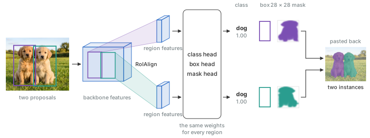
Semantic segmentation produces one class map for the image. Instance segmentation further distinguishes individual objects: two dogs need two separate masks, even though they share a class. Mask R-CNN builds on the object proposals of Faster R-CNN (Chapter 4), adding a mask-prediction branch alongside classification and bounding-box regression [8].

For each region of interest, the network extracts a small spatial feature map from the shared backbone features. The classification head predicts the object’s class, the box head refines its bounding box, and a small fully convolutional mask head predicts its shape. Keeping spatial structure in the mask head allows its output to describe where the object lies within the region.

Figure 6.21: Detection locates the individual objects, and the mask head predicts their shapes. The backbone runs once over the photograph, and RoIAlign takes each proposal’s features from that shared map. The same heads then produce a class, a box and a 28 × 28 mask for each dog. Resized and placed in the image, the masks give two instances of one class. Real Mask R-CNN output on a generated image, from figures/runs/ch06_runs.py.

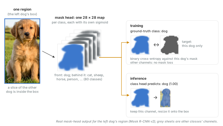
In the original class-specific design, the mask head produces one mask channel per object class. Each channel uses a sigmoid to predict whether each position belongs to the object. These channels do not compete through a softmax: the classification head already handles the choice of class.

During training, a region matched to a ground-truth object receives a binary mask target for that particular instance. Binary cross-entropy is applied only to the mask channel for the object’s ground-truth class; the other mask channels receive no mask loss for that region. At inference, the predicted class selects which mask channel to keep. The selected mask is resized to the detected box and placed back into the image.

This differs from semantic segmentation. There, each pixel chooses among classes. Here, the chosen mask answers a binary question: does this position belong to this particular object? Another dog visible in the region is not part of the target instance’s mask.

Figure 6.22: The mask head produces a 28 × 28 map for every class, each with its own sigmoid, but uses only one per region. In training, the ground-truth class selects the channel that the loss compares with the target mask; at inference, the predicted class selects it. The target drawn is Mask R-CNN’s own mask for this dog, standing in for an annotation. Real Mask R-CNN logits on a generated image, from figures/runs/ch06_runs.py.

6.6.1 RoIAlign

Predicting an object’s class can tolerate some spatial imprecision. Predicting its boundary is more sensitive: a small displacement can move the mask from the object onto its surroundings.

RoI pooling (Section 4.3) introduces this imprecision by rounding the region’s coordinates to the feature grid and rounding again when dividing it into bins. The extracted features therefore describe a slightly altered region. Because backbone features are spaced several input pixels apart, a small rounding error on the feature map can represent a noticeable displacement in the image.

RoIAlign keeps the fractional coordinates of the region and its bins. It samples features at specified positions within each bin, using bilinear interpolation between neighbouring feature-map values, then aggregates those samples. This preserves the alignment between the requested region and the features supplied to the prediction heads [8].

Figure 6.23: Place a fractional-coordinate box over a feature grid. Toggle between RoI pooling and RoIAlign, showing the rounded boundaries in one and interpolation points in the other. Move the box slightly and inspect how the extracted features change. One idea: accurate masks require features sampled from the intended locations.

The mask head still predicts on a fixed spatial grid within each region. Resizing this mask over a large object does not create additional boundary detail, so fine structures can remain difficult to represent even when the region features are accurately aligned.

Mask R-CNN produces masks for individual objects, leaving stuff such as grass and sky unlabelled. A panoptic system can combine these instance predictions with a semantic branch, resolving overlaps to give each pixel one final label and assigning instance identities to thing pixels. Panel (c) of Figure 6.1 shows the result such a system aims for, here produced by a single model, Mask2Former. Models of that kind are the subject of Chapter 10: they predict a set of masks directly, producing semantic and instance-style outputs through one prediction mechanism.

6.7 A U-Net is what you train it to be

U-Net’s encoder, decoder and skip connections are useful beyond segmentation. They provide a way to combine broad context with spatial detail and produce an output arranged on a grid. What that output means depends on the task we train the network to perform.

Three choices connect the architecture to a task: the output representation, which determines what each output value means; the training pairs, which show the desired relationship between input and target; and the loss, which measures how far the prediction is from that target. For multiclass segmentation, the outputs are class scores at each pixel, the targets are label maps, and the loss is per-pixel cross-entropy.

Task	Input → target	Output and training objective
Segmentation	Photograph → class-label map	Class scores; per-pixel cross-entropy
Denoising	Noisy image → clean image	Colour intensities; a reconstruction loss such as mean squared error
Colourisation	Greyscale image → colour image	Colour components, such as two chroma channels alongside the input luma (Section 1.1.4); a reconstruction loss such as mean squared error
Depth estimation	Photograph → depth map	One depth value per pixel; a suitable regression loss
Super-resolution	Low-resolution image → higher-resolution image	Colour intensities on a finer output grid; an appropriate upsampling path and reconstruction loss

These tasks can share the same encoder–decoder design, but the input channels, output head and required output resolution may differ. The loss also influences the kind of prediction the network learns. For example, when several colours or fine textures are plausible, mean squared error can favour their average, producing muted colours or smooth detail.

Figure 6.24: A U-Net can be adapted to four tasks: segmentation, denoising, colourisation and super-resolution. Each column shows a training pair made from our photograph, the input above the target, with the output representation and the loss below. These are training pairs, not model outputs.

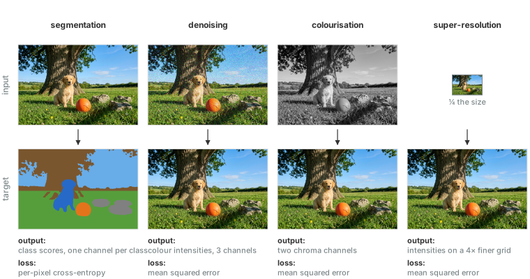
Skip connections are particularly useful when the output must preserve spatial structure from the input. In denoising, the object boundaries should remain in the same places while the noise is removed. Encoder features passed through the skips give the decoder access to local detail that might otherwise be lost during downsampling. They can also carry noise, so the decoder must learn which information to retain.

Lab 6 explores this flexibility by adapting a segmentation U-Net into a denoiser. The encoder–decoder structure remains, while the output head is adjusted to predict image intensities, the targets become clean images, and the loss becomes mean squared error.

Exercises

1. What does the output represent? An image contains two overlapping dogs standing on grass. Describe the output required for semantic, instance and panoptic segmentation. Explain how each represents the two dogs and the grass, and whether its output segments may overlap.
2. When accuracy hides failure. An image contains 100 pixels: 20 object pixels and 80 background pixels. Compare three predictions: (a) every pixel is background; (b) all object pixels are found, but 20 background pixels are also labelled as object; (c) half the object pixels are found, with no false positives. Compute pixel accuracy, object IoU and mean IoU over the two classes. Explain why the metrics give different impressions. What distinction between over-segmentation and under-segmentation is lost when reporting object IoU alone?
3. Finding objects versus outlining them. A class has six ground-truth segments. A model predicts seven segments, with four valid matches at IoUs of 0.90, 0.85, 0.62 and 0.55. Compute SQ, RQ and PQ using the chapter’s definitions. Compare this with a model that finds all six segments at IoU 0.55, with no false positives. Explain what SQ and RQ reveal that PQ alone does not.
4. From a classifier to a dense predictor. A dense layer reads a \(2 \times 2\) feature map with three channels and produces four outputs. Describe the equivalent convolution: its kernel size, input channels and output channels. Explain why the weights can be reused unchanged. What happens when it receives a larger feature map? Why can the resulting fully convolutional network still produce a coarse prediction?
5. Why U-Net needs more than upsampling. Sketch an encoder–decoder with skip connections. Trace the information used to predict a thin object boundary. Explain what the upsampled decoder features and the encoder skip features each contribute. Show how concatenation differs from addition at one join, and explain why neither operation guarantees an accurate boundary.
6. Wide context, dense evaluation. On a small grid, draw the sampling positions of a \(3 \times 3\) convolution with dilation one and dilation two, both at stride one. Mark two neighbouring output positions. Explain why the second kernel samples farther apart but still produces dense outputs. Then explain how reducing downsampling affects computational cost, why ASPP uses several dilation rates, and why very large dilation does not replace global pooling.
7. One mask for one instance. A proposed region contains one target dog and part of another dog. Describe the outputs of Mask R-CNN’s class, box and mask heads. What should the target dog’s binary mask include? Explain which mask channel contributes to training, how a channel is selected at inference, and why the mask head uses sigmoid rather than a softmax across classes.
8. Why alignment matters. Draw a region whose boundaries fall between feature-grid positions. Illustrate how RoI pooling changes those boundaries and how RoIAlign samples the original region. Explain why this difference matters more for an accurate mask than for recognising the object’s class. Does RoIAlign remove the limitations of predicting a mask on a fixed spatial grid?
9. Give U-Net another task. Adapt a multiclass segmentation U-Net for colour-image denoising. Specify the input–target pairs, output channels, suitable output activation and loss. Explain what can remain unchanged and how skip connections may help—or carry unwanted information. Finally, identify the additional output-resolution requirement for super-resolution.

Lab 6

Lab 6: a U-Net for pet-versus-background segmentation on Oxford-IIIT Pet; a comparison with a pretrained Mask R-CNN; then the denoising coupling — same U-Net, MSE loss, noisy-to-clean.

Open in Colab

Further reading

• Long, Shelhamer, and Darrell [3] — FCN; the skip ablation compares FCN-32s, FCN-16s and FCN-8s on one table of mean IU.
• Ronneberger, Fischer, and Brox [4] — U-Net; section 3 defines the border-distance weight map that separates touching cells.
• Chen et al. [6] — DeepLab; atrous convolution stated carefully, and the CRF while it was still there.
• Chen et al. [7] — DeepLabv3; the ASPP and output-stride ablations, and Table 7 for the result without a CRF.
• He et al. [8] — Mask R-CNN; Table 2 compares RoIAlign with RoI pooling and independent mask sigmoids with a softmax across classes.
• Kirillov et al. [1] — panoptic segmentation; the metric, and the argument for needing one.
• Odena, Dumoulin, and Olah [5] — checkerboard artefacts; why kernel size not divisible by stride produces them, and why resize-then-convolve avoids the pattern.

References

[1]

A. Kirillov, K. He, R. Girshick, C. Rother, and P. Dollár, “Panoptic segmentation,” in IEEE/CVF conference on computer vision and pattern recognition (CVPR), 2019, pp. 9404–9413. doi: 10.1109/CVPR.2019.00963.

[2]

D. C. Cireşan, A. Giusti, L. M. Gambardella, and J. Schmidhuber, “Deep neural networks segment neuronal membranes in electron microscopy images,” in Advances in neural information processing systems (NeurIPS), 2012, pp. 2843–2851.

[3]

J. Long, E. Shelhamer, and T. Darrell, “Fully convolutional networks for semantic segmentation,” in IEEE conference on computer vision and pattern recognition (CVPR), 2015, pp. 3431–3440. doi: 10.1109/CVPR.2015.7298965.

[4]

O. Ronneberger, P. Fischer, and T. Brox, “U-Net: Convolutional networks for biomedical image segmentation,” in Medical image computing and computer-assisted intervention (MICCAI), 2015, pp. 234–241. doi: 10.1007/978-3-319-24574-4_28.

[5]

A. Odena, V. Dumoulin, and C. Olah, “Deconvolution and checkerboard artifacts,” Distill, 2016, doi: 10.23915/distill.00003.

[6]

L.-C. Chen, G. Papandreou, I. Kokkinos, K. Murphy, and A. L. Yuille, “DeepLab: Semantic image segmentation with deep convolutional nets, atrous convolution, and fully connected CRFs,” IEEE Transactions on Pattern Analysis and Machine Intelligence, vol. 40, no. 4, pp. 834–848, 2018, doi: 10.1109/TPAMI.2017.2699184.

[7]

L.-C. Chen, G. Papandreou, F. Schroff, and H. Adam, “Rethinking atrous convolution for semantic image segmentation,” arXiv preprint arXiv:1706.05587, 2017, Available: https://arxiv.org/abs/1706.05587

[8]

K. He, G. Gkioxari, P. Dollár, and R. Girshick, “Mask R-CNN,” in IEEE international conference on computer vision (ICCV), 2017, pp. 2961–2969. doi: 10.1109/ICCV.2017.322.