4  Object Detection: The Two-Stage Lineage

NoteLearning objectives

• Define the detection task, score it with IoU and mAP, and suppress duplicates with NMS
• Follow the R-CNN → Fast R-CNN → Faster R-CNN arc as a sequence of removed bottlenecks
• Explain region proposal networks and feature pyramids

Skills ladder. Implement IoU and mAP by hand once, before ever trusting a library’s version. Set thresholds on validation data, never on the test set you intend to quote.

Classification answers what; detection answers what, where, and how many.

This third question creates a structural break from the models we’ve seen so far, which can only produce a fixed number of outputs. Figure 4.1 demonstrates this.

Figure 4.1: The scores in both panels are illustrative rather than an actual model’s output, with Figure 4.2 below being the measured version. (a) Classification scores a fixed list of classes over the whole image and returns a score for each class, regardless of what the image contains. Of the top five illustrated, two describe the dog and disagree about its breed, one is the tree, and one is the ball; nothing in the output says where any of them is, or that there is one of each. Most importantly, all of these responses appear in the image and might not be considered incorrect. (b) Detection returns one entry per object, with each entry consisting of a box, a class, and a score.

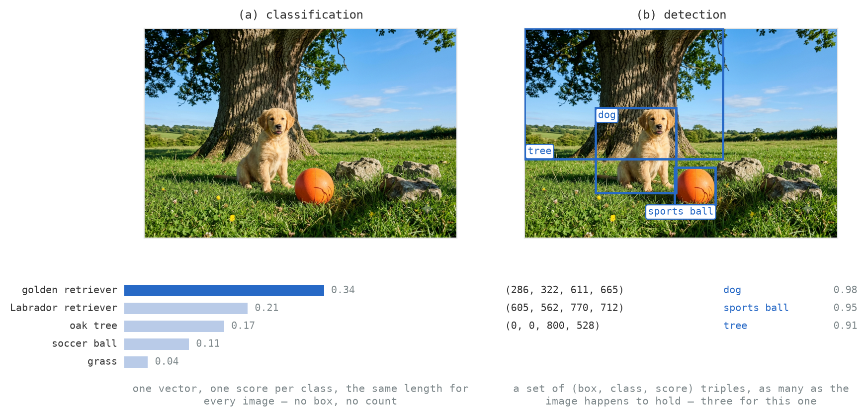
A classifier’s head produces a fixed-length vector, one score per class, the same length for every image. An object detector has to produce a set whose size we do not know in advance: no objects in one photograph, two in the next, forty in the one after that.

Every architecture considered in this chapter turns this variable-length set problem into a fixed-size problem, which we can address with the architectures of the last three chapters. In the two-stage lineage, models first nominate or propose candidate regions where they think objects may be present, then classify each one. The classifier’s output is fixed-length as before, and the variable length problem has shifted to the component that proposes regions.

The four designs that follow are a sequence of removed bottlenecks, and in each case, the arithmetic of the bottleneck is the argument for the next design.

4.1 Object Detection, Metrics, and NMS

A detection is a bounding box, a class, and a score. The bounding box is an axis-aligned rectangle defined by four pixel coordinates in the input image, and it has three common encodings. The corner form \((x_1, y_1, x_2, y_2)\) specifies the top-left and bottom-right corners. This is the most convenient representation to calculate the IoU metric, presented later in this section. The centre form \((x, y, w, h)\) gives the centre point of the box, with a width and a height. The box regressors from Section 4.2 onwards use this representation, because a location correction has to be measured against something: a translation (in units of the box’s own width/height) and a scaling (as a log ratio) mean the same thing at every scale, while two independently regressed corners do not. The third form, which COCO’s annotations use, is \((x_1, y_1, w, h)\): the same top-left corner as the first form, followed by a size rather than a second corner.

NoteBox coordinate pitfalls

Detection code carries all three and often converts between them. Torchvision’s box_convert names them xyxy, cxcywh and xywh, each used where its arithmetic is most natural. The last two are the ones to watch out for. Both read as x, y, then a width and a height, and nothing in a file, a tensor, or a debugger can distinguish them. Mistaking cxcywh for xywh, or vice versa, leads to offsets of w/2 and h/2 that can be difficult to trace.

The class is one label from the closed label set that the detector was trained on. The score is the detector’s confidence in that pairing, a number between 0 and 1 (typically from a softmax). The output for an image is a list of those triples: [(box_location_0, class_0, score_0]), (box_location_1, class_1, score_1])...].

Figure 4.2 shows the output of a real detector on our image. It finds both the Ball and the Dog with scores of 0.999 and 0.996, respectively. It also returns seven other boxes. The calculations that follow later in this chapter use this set of annotations.

Figure 4.2: A real run of torchvision’s Faster R-CNN R50-FPN v2. Gold, dashed: the two ground-truth boxes drawn by hand for this book, the dog at \((286, 322, 611, 665)\) and the sports ball at \((605, 562, 770, 712)\). The nine numbered boxes are every detection with a class score above 0.05: blue where the class agrees and the overlap clears 0.5, grey where it does not. The orange scores an IoU of 0.976 against the ball’s ground truth, localising it better than the correct sports-ball detection does, but a match requires the class to agree. Four more are stacked on one rock, calling it a teddy bear, a bird, a sheep and a bear, and one is a bird on the rock behind it at 0.499 with a second over the same patch at 0.100.

Nothing has gone wrong. Those seven boxes are what this detector produces whenever the score threshold is low enough to keep them, and the usual practice is to discard them based on a higher threshold.

4.1.1 Intersection over union

Deciding whether a predicted box is the same object as a ground-truth box needs a metric. Detection benchmarks typically use intersection over union (IoU): the area the two boxes overlap, divided by the area of their union.

\[ \mathrm{IoU}(B_p, B_{gt}) \;=\; \frac{\lvert B_p \cap B_{gt} \rvert}{\lvert B_p \cup B_{gt} \rvert} \]

It runs from 0 for disjoint boxes to 1 for identical ones, and it is scale-free: multiply every coordinate of both boxes by three (i.e. scale the image and detections by three), and the ratio does not change, because both areas grow by a factor of nine.

What do you think a reasonable threshold is for deciding whether two boxes overlap sufficiently? Use Figure 4.3 to build some intuition.

Figure 4.3: Intersection over union, by hand. The widget opens with the answer hidden: blue is yours to drag and resize, and the exercise is to put it where you would draw the box around the dog before anything is scored. Show ground truth then reveals the gold box drawn by hand for this book, scores your placement against it, and keeps that score, so you can see what your eye was worth before you began adjusting. Guess the number first. Most people are surprised by how low a box that looks right scores, and by how much of the union sits outside the object. After that, the shaded region is the intersection, the dashed border is the union, and the readout gives both areas and their ratio. Find the smallest shift that takes a box from 0.51 to 0.49, then switch the chip to 0.75 and 0.90, and find that edge again to see how little room the stricter thresholds leave. The detector’s box is what Faster R-CNN actually returned here, within four pixels of the gold box on every edge.

PASCAL VOC set the threshold for a correct detection at 0.5: “the threshold of 50% was set deliberately low to account for inaccuracies in bounding boxes in the ground truth data,” since a box around a non-convex object is subjective and a person with their arms and legs spread has no single right rectangle [1]. It is a convention and may vary by image domain and application.

4.1.2 Non-maximum suppression

A single object can produce many correct boxes, each slightly offset from the others. Figure 4.4 shows every box this detector proposes for one animal in the book’s photograph, with suppression switched off.

Figure 4.4: Clusters of overlapping boxes. All of these bounding boxes (blue) are output by the detector for the same object, the dog in the standard scene. Before suppression, slightly offset boxes with similar class and confidence often crowd around the true object (gold dashed). The same cluster, sometimes dozens per object, explains why non-maximum suppression is needed.

A detector evaluates a densely packed set of overlapping candidate regions, which means that when a predicted box closely matches the true object, plenty of other candidates will almost coincide with it. As a result, detections of the same real object typically arrive as clusters of nearly identical boxes. For example, with non-maximum suppression turned off and a score threshold of 0.05, this detector outputs 38 boxes marked dog our image. Of the dog boxes, all 37 other boxes overlap the top-scoring dog detection at an IoU greater than 0.5, and 29 overlap it above 0.9. These boxes are essentially duplicates of a stronger scored detection.

Non-maximum suppression (NMS) removes them, greedily, one class at a time so that we do not return multiple detections for a single object.

ImportantGreedy NMS

Given the detections of a single class and a threshold \(\tau\):

1. Sort the detections by score, highest first.
2. Move the highest-scoring detection still in the queue to the output.
3. Delete every remaining detection whose IoU with it exceeds \(\tau\).
4. Repeat from step 2 until the queue is empty.

The cost is \(O(n^2)\) box comparisons in the worst case, where \(n\) is usually a few hundred after score thresholding.

Applied to the 38 candidate dog boxes of Figure 4.4 at the usual \(\tau = 0.5\), this retains exactly one.

Figure 4.5 shows a scenario with two objects of the same class. Using only one dog can illustrate the need for suppression, but not its purpose: with a single object, an algorithm that removes overlapping boxes behaves like one that simply selects the highest-scoring box. The distinction only appears when multiple objects are present and both should remain. Two generated puppies demonstrate which boxes are removed, and which must stay.

Figure 4.5: Four boxes, two puppies, one class. Two boxes sit on each puppy: a tight one and the sort of offset near-duplicate a dense detector emits alongside it. Step takes the highest-scoring box still in the queue, keeps it, and prints the overlap it measures against every box left, deleting those above \(\tau\). At \(\tau = 0.70\) two rounds leave two boxes, one per puppy. Both ends of the trade-off above are reachable here: at 0.90 the duplicates survive and each puppy is reported twice, while at 0.03 box A’s faint overlap with the other puppy’s boxes is enough to delete them, and one box comes back for two animals. Every overlap is computed from the box coordinates. The photograph is generated rather than taken with a camera, and the four boxes were drawn by hand to stand in for a detector’s output.

Both of those outcomes turned on a number that was chosen rather than derived. Set \(\tau\) too high and duplicates survive, which is the failure Figure 4.5 shows at 0.90. Set it too low and the algorithm starts deleting boxes that belong to different objects, which that scene cannot show at any sensible threshold, because its two puppies sit far enough apart that their correct boxes barely overlap at all. The second failure needs neighbours close enough that the right answer for one already covers part of the other. Two people standing shoulder to shoulder can be marked by two equally sized boxes offset by half their width, which overlap at an IoU of exactly \(1/3\): a threshold of 0.3 deletes one of them, and 0.4 keeps both. Nothing in the image says which side of that line to stand on, and no gradient reaches it, so the value is set by hand and checked on held-out data.

Figure 4.6 is that case. It moves the same four boxes onto two puppies sitting against each other, where the overlap between the two correct boxes is no longer negligible.

Figure 4.6: Two objects, close enough to be confused for one. The boxes are the same four as Figure 4.5 and the algorithm is unchanged; only the spacing differs. Because the puppies touch, the two correct boxes, one per animal, already overlap at 0.334, near the \(1/3\) of the shoulder-to-shoulder case above. At \(\tau = 0.50\) that sits comfortably below the threshold and both survive. At \(\tau = 0.30\) it does not, and C is deleted: not as a duplicate of anything, but for sitting too close to its neighbour, leaving one box for two animals. At \(\tau = 0.40\) both are kept again. The scene chip switches back to the separated pair, where the same thresholds do nothing of the kind.

The deletion is final. NMS runs after the network, on boxes and scores alone; it has no gradient, and nothing downstream can recover a box it removed. Soft-NMS decays the scores of overlapping boxes rather than deleting them, for exactly that reason [2].

Back on our default image, running NMS per class has a visible consequence in Figure 4.2. The four spurious boxes on the rock overlap each other at an IoU above 0.96, and the orange sits on the sports ball at an IoU of 0.956. Same pixels, different labels, so nothing suppresses anything. Figure 4.7 runs the algorithm on the unsuppressed candidates, one deletion at a time.

Figure 4.7: Greedy NMS on real boxes, in the same three phases as Figure 4.5. The widget holds the 59 candidates this detector produces for the two classes actually in the scene, with suppression switched off. Press step repeatedly: one press selects the highest-scoring survivor, then each press measures it against one more candidate, greying its bar if it dies, and a final press carries out the deletions. The middle phase is the one to watch, because it is where per class stops being a footnote. The winning sports ball box is measured against 20 other ball candidates and against none of the 38 dog candidates, which are drawn pale and dashed and sit through the whole round untouched. Switch to any class and the same round measures against all 58, which is the comparison the rule exists to prevent. Predict the survivor count at 0.5 before running it, given that the scene holds two objects. Then find the threshold at which the first duplicate gets through, and say which of the two classes falls apart first.

4.1.3 Precision, recall, and the score threshold

With IoU available, we can assign detections to ground-truth boxes and count successes and failures. The procedure is greedy, working down the score ranking, and its one subtlety is that a ground-truth box can be claimed only once: a second detection of an already-claimed object is a false positive, not a bonus. The VOC benchmark handled “5 detections for one object” as “1 correct detection and 4 false detections,” and placed the responsibility for suppression on the detector rather than the evaluation protocol [1].

TipDetection Matching Algorithm: Step-by-Step

Given a set of detected boxes (with scores) and ground-truth boxes for an image, the standard evaluation protocol assigns detections to ground-truths as follows:

1. Sort detections by confidence score, from highest to lowest.

2. For each detection in order:

   • Find the ground-truth box of the same class with the highest IoU (Intersection-over-Union) with this detection, among those still unclaimed.
   • If that IoU is at least the threshold (e.g., 0.5), assign this detection as a True Positive (TP), and mark that ground-truth box as “claimed”.
   • If no such ground-truth exists or IoU is below threshold, this detection is a False Positive (FP).

3. Any ground-truth box not matched by any detection is a False Negative (FN).

Special caution: As each ground-truth box is removed after being “claimed”, if multiple detections overlap with the same ground-truth box, only the first to claim it is a True Positive; the rest are False Positives. VOC counted “5 detections of a single object” as “1 correct detection and 4 false detections”, and said that filtering them was the detector’s job, not the benchmark’s [1].

NoteVOC matches differently, and almost never visibly

That is COCO’s rule, and it is the one this book uses throughout. VOC’s differs in a single step: it takes the box a detection overlaps most whether or not it has been claimed, and then asks whether that box is free. A detection whose best match is already taken is a false positive under VOC; under COCO it falls through and claims the next-best box still available.

The two can only disagree when a detection’s best match is taken and it clears the threshold on a free box of the same class — which needs at least two objects of one class close enough to compete for the same detection. Evaluated over all 4,952 images of the VOC 2007 test set with the detector this chapter uses, the whole difference is worth 0.0001 of mAP@0.5: 0.8967 under COCO’s rule against 0.8966 under VOC’s. Every other figure in Section 4.1.3 is identical to four decimal places under both.

Two things follow. Reading either evaluator’s source, the skipped-if-claimed test is a single line and easy to miss, so it is worth knowing which one you are looking at. And a number that differs from a published one in the fourth decimal is more likely a protocol difference than a mistake in your code.

Non-maximum suppression is what prevents that last case from inflating the count. It runs before evaluation, not after, so the 59 candidates in Figure 4.7 are reduced to two by the time they reach the matcher; the other 57 duplicates are never evaluated. Suppression alleviates the issue but does not eliminate it because it is applied per class, the orange on top of the sports ball in Figure 4.2 remains unaffected and is, rightfully, counted here as a false positive.

Precision is the fraction of detections that were right, \(\mathrm{TP}/(\mathrm{TP} + \mathrm{FP})\): of all the dogs we predicted, what proportion were correct?

Recall is the fraction of objects that were found, \(\mathrm{TP}/(\mathrm{TP} + \mathrm{FN})\): of all the actual dogs in the image, what proportion of them did we find?

The score threshold is the classification confidence below which detections are discarded, and it trades one against the other.

4.1.4 Average precision

The score threshold determines the balance between precision and recall. Raising the threshold requires the model to be more confident before signalling a detection: this cuts out weak guesses, so precision improves, but it also removes some correct but less confident detections, causing recall to fall as objects go unfound. Lowering the threshold has the opposite effect: the detector accepts more uncertain predictions, so it recovers missed objects and raises recall, but at the cost of admitting more false positives, which lowers precision. Raising the threshold cannot buy recall, and lowering it usually costs precision — but not always: when a newly admitted detection finds an unclaimed object, both rise together, which is exactly what the last row of Table 4.1 does. The trade-off is a tendency of the sweep, not a law of each step, which is why quoting performance at a single threshold says as much about the chosen threshold as about the detector itself.

Varying the threshold from 1 down to 0 traces out a curve that captures the trade-off between precision and recall. As the threshold decreases, additional detections are included, so recall can only increase, since more true objects may be found. Precision, on the other hand, generally steps downward each time a newly admitted detection turns out to be a false positive. This relationship forms the precision–recall curve, illustrated in Figure 4.8, with each point labelled by the threshold at which it is reached.

There are only five thresholds worth testing, each just below a detection score, since detections are included or excluded only as the threshold crosses these values. Between these points, nothing changes; the sweep yields five distinct operating points, which are all shown in Table 4.1.

Table 4.1: Every operating point for the five detections in Figure 4.8. kept is the number of detections with scores at or above the current threshold, and recall is out of three objects. Precision drops from 1.000 to 0.500 as the two false positives are included, then climbs to 0.600 in the final row when the weakest detection of the five discovers the third object, making this the only place in the sweep where lowering the threshold improves both precision and recall.

score threshold	kept	TP	FP	precision	recall
0.99	1	1	0	1.000	0.333
0.95	2	2	0	1.000	0.667
0.90	3	2	1	0.667	0.667
0.50	4	2	2	0.500	0.667
0.10	5	3	2	0.600	1.000

Each threshold picks out a different point on the precision–recall curve. Here, we have three objects (all the same class) and five detections, the same ones tallied in the table above. As you drag the threshold slider, \(\tau\), through the widget, you’ll see the panels shift in sync: detections with lower scores fade from the photo, any object left unclaimed is highlighted as missed, the true and false positive counts (and the corresponding precision and recall values) update for what remains, and the active spot moves along the curve. The curve itself never changes; it is drawn once for all possible thresholds. Where you stand on it is all about your choice of threshold. That’s why average precision, represented by the shaded area under the curve, is a property of the detector as a whole, while actual precision and recall depend on the specific threshold you set.

It’s helpful to check the extremes. At \(\tau = 0\), every detection, good or bad, is included, so all three objects are found, but two detections are counted as wrong. Raise the threshold just past 0.10: now the weakest detection disappears, and with it, puppy 3 is missed, dropping recall to 2/3. From there, no amount of threshold fiddling will bring that missed object back: raising the threshold always removes detections, never adds them. Push \(\tau\) to 1 and everything is filtered out; no detections remain, so precision becomes 0/0: undefined, not zero.

Figure 4.8: Notice also what these panels can’t show: there’s no “true negative” count. The detector never tells us how many boxes it could have predicted but didn’t, so accuracy, the familiar metric from classification, does not translate to detection tasks. Here, everything shown is based on hand-drawn boxes over a generated image, and every overlap, count, and metric is computed directly from coordinates.

The area beneath that curve is called average precision (AP). It is the average of the detector’s precision across its entire range of operating thresholds, rather than at a single point. Precision and recall alone always depend on the threshold you pick, and what “the right threshold” is will change depending on where or how the model is used. A traffic survey and a pedestrian crossing (as in exercise 7) might need very different settings, even with the same detector. Average precision sidesteps this by folding the threshold out of the equation entirely: two detectors can be compared fairly, without having to agree first on how conservative or adventurous they should be.

mAP, mean Average Precision, takes that one step further by averaging AP across all classes. The benchmark scores each class separately, matching every dog detection only to dog boxes, so that rare classes aren’t overwhelmed by common ones. It then computes the mean over all per-class AP values. This mean is unweighted, so a class that barely appears counts just as much as one that shows up thousands of times in the overall figure. That’s a deliberate choice, with trade-offs, and Section 4.1 will explore its implications later in this section.

NoteThree ways to measure the area, and how they differ

The unprocessed precision–recall curve zig-zags: each false positive causes a dip in precision until a true positive lifts it again. Before calculating the area under the curve (AP), all three major conventions first smooth it by interpolating upward, replacing the precision at recall \(r\) with the highest precision observed at any recall \(\ge r\). After this, the area is computed, but each benchmark does so slightly differently. VOC 2007 takes the mean of the interpolated precision at eleven discrete recall points, \(\{0, 0.1, \dots, 1\}\) [1]; VOC 2010 and later instead integrate the curve exactly; COCO samples it at 101 equally spaced points, \(\{0, 0.01, \dots, 1\}\). For the six detections in exercise 2, these protocols yield AP scores of 0.682, 0.6875, and 0.691 on identical predictions. The differences are small but real, which is why an AP value, if reported without its scoring protocol, cannot be fairly compared.

WarningThe library will not give you the benchmark’s number

All three of the major detection conventions rely on interpolation. However, the function most people reach for does not follow suit. sklearn.metrics.average_precision_score describes itself as the weighted mean \(\mathrm{AP} = \sum_n (R_n - R_{n-1}) P_n\), and explicitly notes, “this implementation is not interpolated and is different from computing the area under the precision-recall curve with the trapezoidal rule, which uses linear interpolation and can be too optimistic.” Earlier versions of the library actually used linear interpolation, but changed course after version 0.19.

If you look instead to sklearn.metrics.auc(recall, precision), you get yet another result, one based on the trapezoidal rule that the documentation cautions about. The area toggles in Figure 4.8 illustrate all three approaches using the same five detections: both the interpolated and as-measured methods yield 0.867, since the two dips do not affect recall and therefore do not contribute, while the trapezoidal rule produces 0.850, with its sloped final segment visible in the shaded area. The differences become clearer when a false positive ranks above a true one: on three detections and two objects, ordered wrong-then-right-then-right, the as-measured approach gives 0.583, while interpolation gives 0.667. The interpolated value is never lower, as it always takes the highest running precision.

None of these results is incorrect in itself. But an AP score by itself, without its protocol, is meaningless. AP is as much a statement about the evaluation process as about the detector itself, and results computed by one library cannot truly be compared to a leaderboard generated by another if the protocols differ.

Figure 4.9: Average precision, step by step. For a single class, with five detections and three true objects, process the detections in descending score order. Each detection that claims a ground-truth box not already matched counts as a true positive; all others are false positives. Recall can only increase as you move down the list, while precision drops each time a false positive appears. The three detector presets use the same five scores and match the same three ground-truth objects, differing only in detection order, yet AP ranges from 1.000 to 0.600, showing that ranking is as important as accuracy in this metric. The three area chips represent the conventions described above, each computing AP slightly differently, so they may disagree even on identical predictions.

COCO also goes beyond a single IoU threshold. Its headline AP is calculated by averaging results across ten IoU thresholds, from 0.50 to 0.95 in increments of 0.05, making detectors accountable not just for finding objects but for localising them precisely [3]. This is why AP scores on COCO tend to be lower than those reported for VOC. For example, Faster R-CNN with VGG-16 achieves 21.5% AP on the COCO test-dev split, but scores 42.1% AP on those same images when evaluated at the single VOC-style threshold of 0.5 [4]. Both results stem from identical predictions on identical data; the difference between them is entirely due to the evaluation metric. The further decline from the 73.2% AP reported on VOC 2007 reflects differences in the datasets themselves: COCO contains more objects per image, and a larger proportion of small objects.

Sweeping the threshold, step by step: the widget sorts the 59 pre-suppression candidates for the dog and the ball, plus the 7 final detections the detector reports for classes the scene does not hold by their confidence scores, and matches them up against the two ground-truth boxes. Try moving the threshold slider: every detection above that line stays visible in the left panel, while your “operating point” walks along the precision–recall curve on the right. The shaded area under the (interpolated) curve, the average precision or AP, does not shift as you adjust the threshold: it’s determined by the full set of predictions, not your settings.

Figure 4.10: Before you start dragging, pause and predict: as you lower the threshold, which metric, precision or recall, can only ever go up? Now drag and see if you’re right. Go ahead and tweak the IoU requirement using the chips: for this photo, you’ll see the precision–recall curve stays exactly the same all the way from 0.50 to 0.95. Why? Both predicted boxes match their ground-truth targets extremely well (with IoUs of 0.971 and 0.976), so raising the bar does not affect them, until you go beyond 0.97, where the ball’s prediction finally gets disqualified. Here, COCO’s much-tougher ten-threshold averaging actually costs this detector nothing, because the boxes are so precise. Of course, it’s that same requirement for pinpoint localisation that drags down the AP for detectors whose boxes are looser or less accurate.

Every threshold you set in detection comes down to a decision about who ends up dealing with the mistakes. If you dial up recall, a human reviewer will have to sift through extra false positives the system lets through. If you optimise for precision instead, the model quietly tosses out detections it isn’t confident about, potentially missing something important. Usually, the burden from these errors doesn’t fall on the same people. The most vulnerable spots are often those classes the model saw little of during training, and real-world difficulties or distribution shifts can make its confidence even shakier. These risks show up only after you deploy, not just in your validation numbers. mAP, for its part, hides all this nuance: by averaging over all classes (and, in the case of COCO, over multiple IoU thresholds), it can reward small, broad improvements while ignoring major losses on the very class you care about most. A benchmark score is not a justification for launching a system. Before you quote a number, ask yourself: which mistakes got lost in the average, and who would have had to deal with them?

4.2 R-CNN: detection by classification

R-CNN is, at its core, quite straightforward: it takes a set of candidate regions in an image and runs a classifier on each one [5].

These regions come from selective search. The algorithm works by first over-segmenting the image into small patches called superpixels, areas of similar colour and texture, using Felzenszwalb and Huttenlocher’s efficient graph-based segmentation. It then continually merges the neighbouring pair that are most alike, based on four handcrafted similarity scores (colour, texture, size, and how fully they “fill” their common bounding box). Every grouping created during this process contributes its own bounding box as a potential candidate [6]. In its fast mode, which R-CNN uses, the method yields about 2,134 boxes per image on the VOC 2007 test set (covering 98% of annotated objects), or 2,147 boxes at 3.79 seconds per image on train+val (where parameters were chosen). This is pure algorithmic logic: every rule is chosen by hand, not learned from data.

For each proposal, R-CNN crops and warps it to a fixed \(227 \times 227\) square, regardless of the original aspect ratio, and feeds it into a CNN that was first pretrained on ImageNet and then fine-tuned for detection. The CNN’s 4,096-dimensional feature vector is then passed through a separate linear SVM for each class (this is the “frozen features” approach from Section 3.4, but here, the backbone is fine-tuned first). A ridge regressor specific to each class also predicts four tweaks to the box: two scale-invariant shifts of the center, and two log-scale adjustments to its width and height [5]. Finally, non-maximum suppression (NMS) eliminates duplicates.

This process consists of three distinct learning steps, all run in sequence, with features written to disk in between: first, fine-tune the network with a log loss; next, extract and cache a feature vector for every proposal in the training set; finally, train the SVMs and regressors. The sheer scale was daunting: Girshick later reported the caching alone cost 2.5 GPU-days for the 5,000 VOC 2007 trainval images, and filled hundreds of gigabytes [7].

Despite this, R-CNN worked wonders. On VOC 2012, it achieved a mAP of 53.3%, over 30% better than the previous best [5]. On VOC 2007, it scored 58.5% using AlexNet as its backbone, and 66.0% with VGG-16, both with box regression added. The whole pipeline is illustrated in Figure 4.11.

Figure 4.11: R-CNN, end to end. The blue boxes are real selective-search output on this photograph. OpenCV’s implementation of [6] returns 2,415 of them here, and sixteen are drawn, spread over the frame, so the scatter shows where the algorithm puts its candidates. The best of the 2,415 reaches IoU 0.74 with the dog box drawn by hand for this book; that is the ceiling every later stage inherits. The box in ink is the one followed across the figure: cropped and warped to \(227 \times 227\) whatever its shape, then a CNN forward pass of its own. A per-class linear SVM scores the 4,096-dimensional fc7 vector; the class-specific ridge regressor reads pool5 instead, which is why its arrow leaves the last convolutional block rather than the vector [5], appendix C. The bracket at the foot is the cost of the design: the backbone runs once per proposal, not once per image.

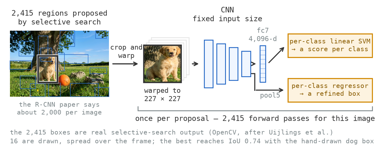
R-CNN’s remaining problem was speed, and the reason was baked into its design. Every one of those (often overlapping) proposals required its own full CNN forward pass. With VGG-16, that added up to 47 seconds per image on a GPU [7]. To process the 4,952 images of the VOC 2007 test set? That’s 65 hours for one evaluation run. The convolution time, run thousands of times on heavily overlapping crops, was by far the biggest bottleneck.

4.3 Fast R-CNN: share the features

Let’s look for the unnecessary repetition here. A convolutional response depends only on the local neighbourhood of pixels, meaning that if you take two crops that both cover that area (well inside their own boundaries), you’ll compute the same feature there both times. (Chapter 2 reminds us that this “equivariance” isn’t perfect due to padding, strides, and the fact that edges behave differently, so crops of the same object can still produce slightly different outputs near the edges. Changing the crop size, or the way it’s resized, adds discrepancies.) Still, in R-CNN, running the network backbone thousands of overlapping times means almost all convolutional work is redundant.

Fast R-CNN fixes this waste: it runs the backbone CNN once, on the whole image [7]. Instead of cropping pixels, it projects each proposal onto the resulting feature map. To do this, it divides the region’s corners by the backbone’s stride (which is 16 for VGG-16’s conv5, the product of four pooling layers), landing the box on precisely the part of the feature map that corresponds to those pixels. Figure 4.12 visually compares this streamlined pipeline to the original.

SPPnet [8] had already shown it was possible to pool proposals from a single feature map calculated for the whole image, but its training could not update the backbone’s convolutional layers, limiting the accuracy of deep backbones [7]. Fast R-CNN introduced end-to-end training for the entire model.

Figure 4.12: The same work, with the convolution run once. Top: R-CNN crops each of the 2,415 selective-search proposals from the photograph and runs the backbone on every crop, warped to VGG-16’s \(224 \times 224\). Bottom: Fast R-CNN runs the backbone once on the whole photograph; each proposal’s corners are divided by the total stride to land on the feature map, and RoI pooling turns whatever rectangle results into a fixed block for the head. The bars on the right count the pixels each backbone convolves per image, 121.2 million against the photograph’s 1.07 million, 113 times fewer. That ratio counts convolved pixels, not run time. The panel at the foot works one real proposal through the projection on a stride-16 backbone: its four edges move 4, 6, 4 and 4 px, against a worst case of half a cell, 8 px.

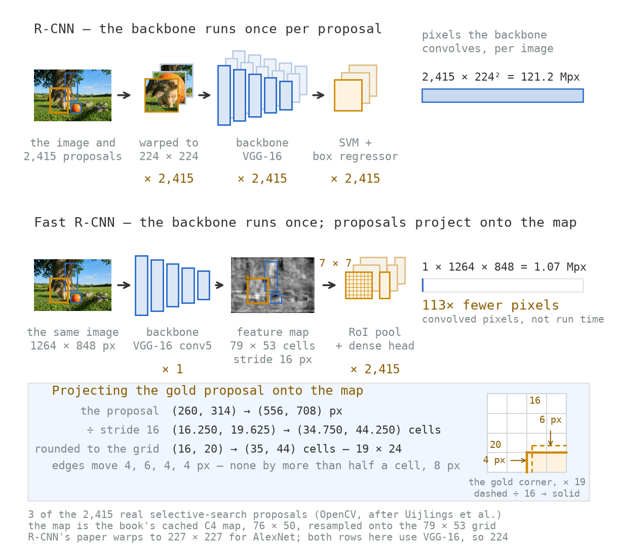
Of course, there’s one wrinkle: even after projecting, these boxes can still have all sorts of shapes, but fully connected (dense) layers need input of a fixed size. That’s where RoI pooling comes in. It divides each projected box, regardless of its actual dimensions, into a fixed \(7 \times 7\) grid, and then max-pools each bin into one value [7]. As a result, every proposal, whether big or small, fat or skinny, gets converted into a neat \(7 \times 7 \times C\) block, suitable for the dense head.

There’s a lot of rounding involved here, and it’s worth seeing what happens in numbers. Take the dog’s bounding box from Figure 4.2, \((286, 322, 611, 665)\), running through a stride-16 map. Divide by 16 to project: \((16.863, 18.986, 36.026, 39.210)\) in feature map “cells.” The system then snaps these to whole numbers: \((17, 19, 36, 39)\). How much did the box move in the image? The edges shift by \(+2.3\), \(+0.2\), \(-0.4\), and \(-3.6\) pixels, and the worst possible shift is half a cell, 8.5 pixels. That snapped box is 19 cells wide and 20 tall, neither neatly divisible by 7. So, for the \(7 \times 7\) grid, we need a second quantisation: for each bin, its start is rounded down, its end rounded up, leading to uneven bins of 3, 4, 4, 3, 4, 4, 3 cells wide for the columns. The two directions of rounding mean neighbouring bins can overlap: for example, bins 1 and 2 both read column 19. In total, 6 of the 19 columns get double-counted, with the narrow bins covering three-quarters of what the wide bins see. The end result is a \(7 \times 7\) grid that’s close, but not quite exactly where we originally wanted it.

Here’s a fun detail: one cell isn’t a “clean” 16 pixels, but 16.96, due to preprocessing. The original \(1264 \times 848\) image is resized to \(800\) pixels tall, then padded out to \(1216 \times 800\) so that every stride divides it. The resulting map is \(76 \times 50\) at stride 16 (in padded coordinates), which actually means each “cell” is \(848 / 50 = 16.96\) pixels in the original. Be sure to project boxes in the right coordinate system! The figures in this chapter use a feature pyramid; specifically, pooling comes from the stride-16 level (P4), but the arithmetic is the same for any stride.

If all you want is a class label, these minor pixel misalignments don’t really matter. But if you need a box placement that’s just right, or per-pixel masks (see Chapter 6), those snap-induced misalignments show up in your results. If your detector’s boxes are always a couple pixels off, this may well be why. The fix is RoIAlign, which does away with both roundings and instead samples features at each bin’s exact real-value position using bilinear interpolation [9]. This improvement matters most for segmentation, but it helps precise detection too; Figure 4.13 shows both approaches side by side.

Figure 4.13: One proposal, projected and pooled. The left panel is the photograph (with a draggable box, or dog, ball, and tiny proposal presets); the center is the model’s real stride-16 feature map (\(76 \times 50\)), showing both the projected and snapped proposal boxes. The right panel shows the \(7 \times 7\) output. Click any bin to see which cells contribute to it. Try the dog first and check the edge shifts; click bins along one row and notice the overlap. For the tiny proposal, with fewer than 7 cells, bins end up reading the exact same cell, so no spatial information is left. Flipping to RoIAlign removes the double-rounding: now, bins sample exactly where instructed, by interpolation.

With feature maps available, there’s no longer any need for separate SVMs and regressors. Fast R-CNN replaces all three of R-CNN’s earlier learning steps with a single network, trained end-to-end using a single loss: a softmax across \(K + 1\) classes (background included), and for each class, four box adjustments in R-CNN’s format. The loss is:

\[ L \;=\; L_{\text{cls}} \;+\; \lambda\,[u \ge 1]\, L_{\text{loc}}, \]

Here, \(u\) is the true class of the proposal; the box regression term is switched off (by the bracket) for proposals labelled background, which have no “true” box to regress to.

NoteSmooth \(L_1\)

For box regression, Fast R-CNN uses a loss that is quadratic for small errors and linear for large ones:

\[ \mathrm{smooth}_{L_1}(x) = \begin{cases} 0.5\,x^2 & \lvert x \rvert < 1, \\ \lvert x \rvert - 0.5 & \text{otherwise,}\end{cases} \]

It treats small mistakes gently (quadratic when \(x\) is small), but switches to linear loss for large errors, so an outlier proposal can only ever nudge the model so hard, rather than blowing up the gradients [7]. At \(|x| = 1\), the two parts connect smoothly.

The results? Accuracy holds, but speed soars. Training VGG-16 for detection drops from 84 hours to 9.5. Testing falls from 47 seconds per image to 0.32, a 146-fold improvement (or 213× with a further SVD trick on the dense head). And, as a bonus, VOC 2007 mAP goes up a hair (from 66.0% to 66.9%) [7]. That 65-hour evaluation? Now 26 minutes.

All these timings skip proposal generation, which now becomes the most time-consuming part. Selective search usually runs on CPU and can take significantly longer than the rest of the trained network.

4.4 Faster R-CNN: learn the proposals

Ren et al. asked why the proposals, alone in the pipeline, were still hand-coded when they could be learned. Here’s the time breakdown for VGG-16 with selective search: 146 ms in the backbone CNN, 1,510 ms for making proposals, and 174 ms for the per-region head. That’s 1,830 ms per image, with a whopping 83% spent on slow, untrained proposals, or about half a frame per second [4].

Yet the features needed to spot “good” regions are right there in the shared feature map. Proposals are boxes with scores, and a box is four numbers, exactly what a tiny convolutional network can emit. So Faster R-CNN introduces the region proposal network (RPN): a lightweight prediction head, reading from the shared feature map and trained seamlessly using ordinary backpropagation.

The RPN comprises three convolutional layers. The first is a bank of 512 filters (256 for smaller backbones), each of size \(3 \times 3\): one filter reads a \(3 \times 3\) window through every channel of the shared map and produces a single number per position, so the bank together produces a 512-dimensional vector at each position. Two branches of \(1 \times 1\) convolutions then read this vector: one has \(2k\) kernels outputting \(2k\) “objectness” scores (two neurons per reference box, a binary object-or-not classification), the other predicts \(4k\) numbers (boxes), where \(k\) is the number of reference boxes at each map position [4]. Importantly, all these convolutions are shared across the spatial map, like the convolutions in the backbone network itself, but here applied to proposing regions instead of classifying. See Figure 4.14 for a diagram.

Figure 4.14: The region proposal network. Top: the shared map is VGG-16’s conv5, \(62 \times 37 \times 512\) at stride 16 for a \(1000 \times 600\) input. A \(3 \times 3\) window of it is read by 512 filters, one number each, giving a 512-dimensional vector, which two \(1 \times 1\) convolutions read, one emitting \(2k\) objectness scores and one emitting \(4k\) box deltas. Bottom: the \(k = 9\) anchors at a single position, drawn to scale on that input, three areas (\(128^2\), \(256^2\), \(512^2\) px) by three aspect ratios (1:1, 1:2, 2:1) with \(w = s\sqrt{r}\) and \(h = s/\sqrt{r}\), and their pixel sizes tabulated beside them. At this centre the \(362 \times 724\) anchor runs past the image edge, and anchors that cross the boundary are dropped during training. Every weight in the diagram is shared across all \(62 \times 37 = 2{,}294\) positions, which carry \(20{,}646\) anchors between them.

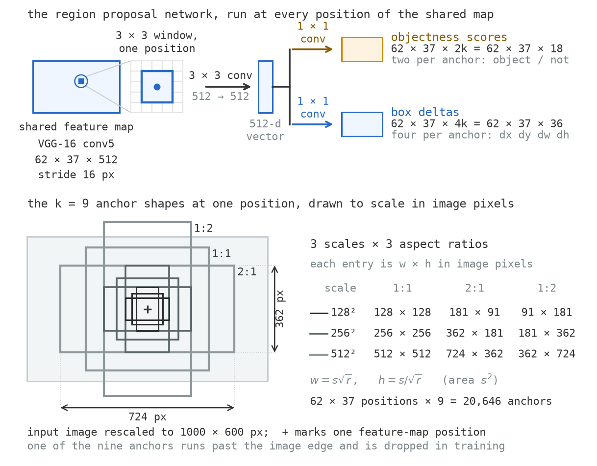
Here, \(k\) is the number of anchors: predefined, fixed boxes centred at each position. In the classic setup, there are \(k = 9\) per position: three different areas (\(128^2\), \(256^2\), \(512^2\) pixels) and three aspect ratios (1:1, 1:2, 2:1) [4]. An anchor isn’t a prediction; it’s a “starter” shape for the network to refine. The RPN regresses each anchor to better fit objects using this familiar parameterisation:

\[ t_x = \frac{x - x_a}{w_a}, \qquad t_y = \frac{y - y_a}{h_a}, \qquad t_w = \log\frac{w}{w_a}, \qquad t_h = \log\frac{h}{h_a}, \]

Here, \((x_a, y_a, w_a, h_a)\) define the anchor’s center and size. The x/y shifts are relative to the anchor’s size, and the w/h changes are in log-space, so the same predicted values have the same meaning at any scale. Compare this to directly predicting absolute pixel coordinates every time, a much harder learning problem. Instead, each anchor only needs to learn how to “nudge” itself, from a sensible starting place, to tightly fit an actual object.

Anchors blanket the image thanks to dense feature maps. For an image of \(1000 \times 600\) pixels on a stride-16 map, the resulting grid is \(62 \times 37\): 2,294 positions, 9 anchors each, about 20,646 anchors for the whole image. (The paper reports that, typically, only about 6,000 survive after excluding those that hang off the edges [4].)

Assigning labels to anchors is based on IoU overlap with ground-truth boxes. If an anchor gets IoU \(\ge\) 0.7 against any ground-truth box, it’s positive (“foreground”); if its IoU is below 0.3 for all, it’s negative (“background”); otherwise, it doesn’t affect training. There’s a third, crucial rule: for each ground-truth box, the anchor that overlaps it most, no matter how low the IoU, is marked positive as well. Why? Because with only 9 fixed shapes per grid spot, some objects are impossible to match closely. If not for this rule, objects with no good anchor nearby would never contribute to training. For instance, an upright pole \(24 \times 420\) pixels in size only reaches 0.196 IoU with the best possible anchor, well below the positive threshold.

For training, the loss is computed over 256 anchors sampled per image, balancing positives and negatives up to 1:1. Since background examples vastly outnumber foreground, this sampling prevents overwhelming the training with negatives [4]. At test time, the RPN’s boxes are filtered by NMS at 0.7 IoU, leaving about 2,000 per image, out of which the top 300 by “objectness” are sent to the detection head for final classification. Figure 4.15 shows this process interactively.

Figure 4.15: Anchors, counted and matched. The grid represents all positions in the feature map at your chosen stride, each with the same nine anchor shapes. Manually count for stride 16, then see how many anchors dangle off the image edge and get pruned before training. Drag the cursor over the grid to show that position’s anchors on the photo. With the paper’s scales, neither object here reaches 0.7 IoU with any anchor, so the “highest-IoU” rule is necessary for them to train at all. The dog covers the area of a \(334 \times 334\) square: adjusting the anchor scale step to \(\sqrt[3]{2}\) starting at 256 lets the dog reach 0.90 IoU (meeting threshold), while the ball (157 pixels) falls from 0.66 to 0.38 and still relies on the extra rule. One set of scales can’t fit every object perfectly, which is the challenge answered in Section 4.5.

With this shared proposal mechanism, the timing improves: 141 ms for backbone, 10 ms for proposals, 47 ms for the head, a total of 198 ms per image (about 5 fps), which is more than 9 times faster than using selective search. And accuracy? It actually improves, rising to 73.2% mAP on VOC 2007 and 70.4% on VOC 2012 (trained with extra data) [4].

Now, the only “hand-designed” part left is NMS (and some knobs: the NMS threshold, anchor shapes, and the cap of 300 proposals). The slowest part remaining is the per-region head, whose computation still scales with the number of proposals, 47 out of the 198 ms per image. Importantly, what’s still tricky for accuracy is handling scale.

4.5 Feature pyramid networks

So what about that scale problem? Using one feature map means one stride, and one resolution. On a stride-16 map, a tiny \(32 \times 32\) object is covered by a mere \(2 \times 2\) cells. Asking RoI pooling to squeeze a \(7 \times 7\) grid from that territory means most bins see repeated values: the finer details get lost. If you try to use a shallower layer for better spatial resolution, you run into a different problem: those early layers have small receptive fields and only simple patterns (edges, blobs), not high-level object features. Tiny objects actually need fine detail and deep features, but standard CNNs put those qualities at opposite ends of the network.

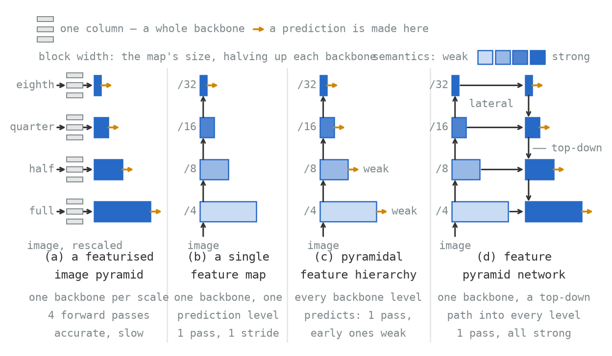
Researchers proposed four design options for dealing with scale, shown side-by-side in Figure 4.16:

• Featurize an image pyramid: resize the input several times and run a full backbone on each, so every scale gets deep features. (Great, but expensive: one pass through the backbone per scale!)
• Predict from a single feature map: fast and efficient, but only works well for objects at the scale matching that map’s stride.
• Predict from all feature hierarchy levels (“pyramidal feature hierarchy”): this reuses backbone work, but the finer, early levels are stuck with weak, low-level features.
• Build a feature pyramid network (FPN): combine the best of both worlds, building a pyramid where every level carries deep features.

Figure 4.16: Four ways to get scale. (a) A featurised image pyramid: resize the input and run the whole backbone on each copy, so every level has deep features, at one backbone pass per level. (b) A single feature map: one pass, predictions from the last map only, which is fast but gives one stride and one scale. (c) A pyramidal feature hierarchy: predict from each stage of the backbone, which adds no backbone passes, but the finest levels are the earliest and their features are the weakest. (d) FPN: one backbone pass plus a top-down path, so every level is both fine and deep. Gold arrows mark where a prediction is made; the fill of each block is how much processing it has behind it, pale for shallow and solid for deep; each block’s width is its spatial size, halving at every step up the column. After Lin et al. [10], figure 1.

FPN’s solution is to add a top-down path alongside the backbone, in addition to reusing all the stages of the network, but enhancing and merging information so that every level, shallow or deep, holds useful features. The backbone’s own “stages” (for ResNet: C2 to C5, at strides 4, 8, 16, and 32) provide the raw maps. The process starts from the deepest map: apply a \(1 \times 1\) convolution to make the number of channels manageable (256), which becomes P5. Then, P4 is made by upsampling P5 by 2× using nearest-neighbour interpolation, adding C4 (also sent through its own \(1 \times 1\) lateral convolution to 256 channels), and then running a \(3 \times 3\) convolution to reduce aliasing. Repeat this for P3 and P2. For the largest scales, P6 is formed by downsampling P5 by 2× (the typical implementation is a \(2\times\) max-pool). Now, every level in the pyramid, from fine to coarse, can be read by the detector head or the RPN. All maps are 256 channels deep, so one set of weights suffices for the prediction head (Figure 4.17 illustrates all this).

Figure 4.17: FPN’s wiring, on a ResNet-50 reading this book’s photograph, resized and padded to \(1216 \times 800\) so that every bottom-up stride divides it. Left, the bottom-up path: the backbone’s own stages, C2 to C5, at strides 4, 8, 16 and 32, so \(304 \times 200\) down to \(38 \times 25\), the maps halving and the channel counts growing upward. Right, the top-down path: P5 is C5 through a \(1 \times 1\) convolution to 256 channels; each level below is the level above upsampled \(2\times\) by nearest-neighbour interpolation, added to a \(1 \times 1\) lateral projection of the matching C map, then passed through a \(3 \times 3\) convolution. P6 is P5 subsampled by 2, drawn here as the \(2\times\) max-pool implementations use: P5’s 25 rows do not halve, and the pool leaves \(19 \times 13\). It is read by the region proposal network only. All levels carry 256 channels, and one head reads them all. The panel at the foot assigns an RoI to a level by \(k = \lfloor 4 + \log_2(\sqrt{wh}/224) \rfloor\), clipped to \(2 \le k \le 5\), and works four box sizes through it.

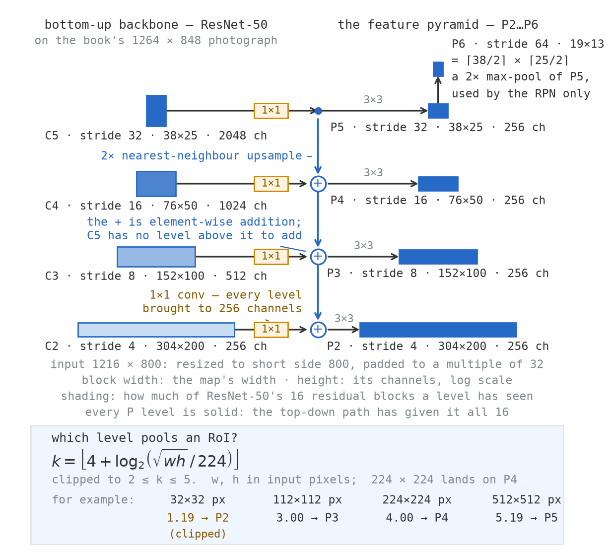
This design is guided by two rules:

• The RPN’s anchors are now spread across all pyramid levels: \(32^2\), \(64^2\), \(128^2\), \(256^2\), and \(512^2\) at P2 through P6, each with three aspect ratios, giving 15 anchor types instead of 9 at a single level. This lets anchor sizes fit image content at different scales.
• Each RoI (proposal) is assigned to a pyramid level according to its size:

\[ k \;=\; \left\lfloor k_0 + \log_2 \frac{\sqrt{wh}}{224} \right\rfloor, \]

with \(k_0 = 4\) [10]. Boxes of \(224 \times 224\) (ImageNet size) go to P4 (stride 16); halve the side and drop a level. The dog from Figure 4.2 goes to P4, the ball (smaller) goes to P3. So, even in a single photo, objects at different scales use different levels, which is the crucial improvement.

And the results fit expectations. On COCO, using a ResNet-50 backbone and predicting only from C4 yields 31.6 AP (minival split), but switching to FPN lifts this to 33.9, and dramatically boosts AP for small objects (from 13.2 to 17.8) [10]. With a deeper ResNet-101 backbone, FPN Faster R-CNN reaches 36.2 AP on COCO’s test-dev at 0.172 seconds per image on a single GPU.

Looking back, Section 1.5 introduced Gaussian pyramids (blurring and downsampling) and Laplacian pyramids (subtracting each level from the upsampled higher one) to let fixed operators find structure at any level. FPN borrows the way Laplacian pyramids are built, going top-down and combining and upsampling at each step, but swaps the details: instead of reconstructing differences, it adds refined features, and doesn’t aim for perfect invertibility, just for the right structure.

4.6 The two-stage template and its costs

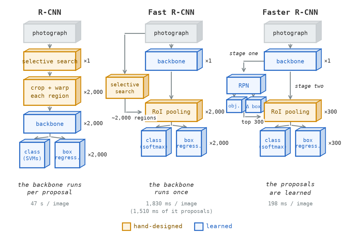
Stepping back, a clear template emerges from these four papers: use a backbone to build shared features, propose regions somehow, and use a head to classify/refine each region. Figure 4.18 draws the three detectors as one pipeline, three times over. In R-CNN, proposals came from a hand-designed module and the backbone was run per region; Fast R-CNN moved the backbone “in front,” so features were shared; Faster R-CNN replaced the proposal generator with a learned head; FPN extended backbone features to cover different object scales. What remains in all four is the “two-stage” idea: nominate regions, then carefully adjudicate.

Figure 4.18: The lineage, one column per design. The same pipeline three times: gold slabs are hand-designed and carry no gradient, blue are learned, and the multiplier beside each is how many times it runs per image. Read left to right, the gold drains out — and the fork moves. Fast R-CNN forks at the photograph: selective search runs on pixels, and its ~2,000 regions meet the backbone’s features at RoI pooling. Faster R-CNN forks at the feature map: stage one is the RPN, emitting objectness and box deltas for every anchor, whose top 300 regions feed the same RoI pooling; stage two is the per-region head. Every design ends the same way, a classification output beside a box-regression output — R-CNN’s are SVMs and ridge regressors, the later two are a softmax and a regression layer of one network. Timings are the papers’ own, quoted earlier, for VGG-16 backbones.

Second-stage processing happens per region. Whatever the head costs in FLOPs gets paid over and over, once per proposal (typically 300 per image), so computation grows with the number of proposals, not the image size itself. If you want to go faster, you can either use fewer proposals, or shrink the head, but both can cost you accuracy.

But the two-stage design has another subtle cost: it has “seams” that gradients can’t cross. RoI pooling introduces (at least) two points of quantisation. The region-selection step picks out which 300 of around 20,000 anchors the head will ever see, by sorting and thresholding, and gradients don’t reach through this. NMS, which deletes duplicate detections, is run after loss calculation, and is again not differentiable. So, a two-stage detector is trained jointly, but it isn’t one smooth, continuous function from pixels all the way to boxes.

The next chapter, Chapter 5, shows what happens if you get rid of stage two: directly predict a class and box at each anchor on the feature map in one fell swoop, and let NMS tidy up. This gives you speed, but opens up new challenges, like class imbalance, that the RPN’s careful sampling had been helping to manage.

Exercises

1. IoU by hand. Given a ground-truth box \((120, 80, 240, 180)\) and a prediction \((160, 80, 280, 180)\) (all in \((x_1, y_1, x_2, y_2)\) format, pixels), calculate:

   • the intersection area
   • each box’s area
   • the union area,
   • and the IoU. The answer should land exactly at the VOC threshold. Then, shift the prediction box 10 pixels to the right (to \((170, 80, 290, 180)\)) and repeat. Now multiply all eight coordinates of the original by 3 and compute again. Explain what (if anything) changed, and why.

2. Precision, recall, and AP. A detector is evaluated on one class across several images. The dataset contains four non-difficult ground-truth objects, G1–G4. The six detections are already ordered by decreasing score. The table gives each detection’s best same-image match; every unlisted IoU is below 0.5.

   Detection	Score	Best match	IoU
   D1	0.95	G1	0.82
   D2	0.90	G2	0.77
   D3	0.80	G2	0.61
   D4	0.70	G3	0.58
   D5	0.60	G3	0.44
   D6	0.50	—	0.09

   Use an IoU threshold of 0.5. A ground-truth object may be claimed only once.

   1. Mark each detection as a true positive or false positive. For every true positive, name the object it claims.

   2. Calculate the running precision and recall after each detection, then sketch the precision–recall curve.

   3. Form the interpolated precision envelope and calculate its exact area. Express the AP as a fraction with denominator 16.

   4. The three false positives have different causes: a duplicate detection, poor localisation, and a detection of background. Identify each one.

   5. What is the highest recall the detector reaches? Explain why it cannot reach 1.

3. NMS traced by hand. You’re given five detections for one class: \(A = (100, 100, 200, 200)\) at 0.92, \(B = (120, 110, 220, 215)\) at 0.85, \(C = (300, 120, 400, 230)\) at 0.71, \(D = (310, 130, 405, 240)\) at 0.63, \(E = (125, 125, 225, 225)\) at 0.55. Calculate the four nonzero pairwise IoUs; then, trace greedy NMS for \(\tau=0.5\) and for \(\tau=0.3\), listing survivors after every step. Box \(E\) overlaps \(B\) at 0.72 yet survives \(\tau=0.5\). Why, in terms of algorithm order? If the true scene has two objects, which threshold “got it right,” and what tradeoff did the other make?

4. Counting anchors. For an input size of \(1216 \times 800\) and stride 16, with 9 anchors per feature-map position, how many positions and how many anchors are there? Now consider the FPN setup: five levels at strides 4, 8, 16, 32, and 64, with one scale and three aspect ratios per level (and rounding up each map’s size as needed). What’s the total number of anchors, and what share comes from the finest level? What does this fraction say about the ratio of positive to negative anchors for an anchor-based detector?

5. RoI projection, with the error in pixels. For a proposal at \((73, 41, 219, 188)\) (stride 16 backbone), compute:

   • the projected corners before and after snapping to whole cells,
   • how far each edge moves in pixels,
   • and the maximum possible movement for any edge, for any proposal. The snapped box is \(9 \times 9\) cells: divide one axis into 7 bins according to real RoI pooling rules (bin starts rounded down, ends rounded up), and list the cells each bin covers and its width. Six bins should be two cells wide, one will be three, and each pair of adjacent bins shares a cell. What effect does reading a cell twice have on the head’s “view” of the object? Which rounding moves a bin boundary furthest?

6. Why the third assignment rule exists. In Faster R-CNN, an anchor is positive if its IoU is at least 0.7 with a ground-truth box, or if it’s the highest-overlapping anchor for that box, whatever the IoU. Take a ground-truth box \((388,190,412,610)\) (a tall, skinny pole; \(24 \times 420\) px). Use only area and aspect ratios to show that none of the usual nine anchors (\(128^2\), \(256^2\), \(512^2\); ratios 1:1, 1:2, 2:1) can hit IoU \(0.7\) here, at any stride-16 position (the best you’ll find is 0.196 after exhaustive search). What happens during training without the third rule, and what would the detector do with poles like this at test time?

7. A threshold, in a deployment. Suppose you’re using a two-stage detector for a traffic survey with a fixed intersection camera, counting vehicles. You control two thresholds: score and NMS IoU. What starting values would you pick for each? For each, describe what happens if you move it up or down. On a day’s new footage, what would you measure to tune them? If you had to set one threshold “wrong,” which would you pick, and would your answer change if the system were tasked to count pedestrians instead?

Lab 4

Lab 4: pretrained Faster R-CNN inference; compute IoU/mAP on a small set; visualise proposals and NMS effects.

Open in Colab

Further reading

• Everingham et al. [1] — the VOC challenge; section 4.2 defines the metric used throughout this chapter, and section 6.2.3 discusses the impact of raising the IoU threshold to 0.5.
• Lin et al. [3] — COCO; the dataset and new metric that replaced VOC’s, and the reason detection “scores” seem to halve after 2015.
• Uijlings et al. [6] — selective search; a look at the craftsmanship and complexity behind hand-designed proposal algorithms.
• Girshick et al. [5] — R-CNN; relevant for its box parameterisation (Appendix C), still foundational today.
• Girshick [7] — Fast R-CNN; see Section 1.1’s plain-spoken summary of R-CNN’s three core weaknesses.
• He et al. [8] — SPPnet; the pivotal intermediate step. Fast R-CNN’s main contribution is making end-to-end training possible.
• Ren et al. [4] — Faster R-CNN; Section 3.1’s explanation of anchors and the experiment table together justify the classic settings.
• Lin et al. [10] — FPN; Figure 1 lays out the four “scale” designs, while their ablation table shows the payoff for each design choice.
• He et al. [9] — Mask R-CNN; read now for RoIAlign, and revisit in Chapter 6 for the full treatment.
• Bodla et al. [2] — Soft-NMS; the case where greedy NMS fails is a subtle test of your algorithm intuition.

References

[1]

M. Everingham, L. V. Gool, C. K. I. Williams, J. Winn, and A. Zisserman, “The PASCAL visual object classes (VOC) challenge,” International Journal of Computer Vision, vol. 88, no. 2, pp. 303–338, 2010, doi: 10.1007/s11263-009-0275-4.

[2]

N. Bodla, B. Singh, R. Chellappa, and L. S. Davis, “Soft-NMS — improving object detection with one line of code,” in IEEE international conference on computer vision (ICCV), 2017, pp. 5561–5569. doi: 10.1109/ICCV.2017.593.

[3]

T.-Y. Lin et al., “Microsoft COCO: Common objects in context,” in European conference on computer vision (ECCV), 2014, pp. 740–755. doi: 10.1007/978-3-319-10602-1_48.

[4]

S. Ren, K. He, R. Girshick, and J. Sun, “Faster R-CNN: Towards real-time object detection with region proposal networks,” in Advances in neural information processing systems (NeurIPS), 2015. Available: https://arxiv.org/abs/1506.01497

[5]

R. Girshick, J. Donahue, T. Darrell, and J. Malik, “Rich feature hierarchies for accurate object detection and semantic segmentation,” in IEEE conference on computer vision and pattern recognition (CVPR), 2014, pp. 580–587. doi: 10.1109/CVPR.2014.81.

[6]

J. R. R. Uijlings, K. E. A. van de Sande, T. Gevers, and A. W. M. Smeulders, “Selective search for object recognition,” International Journal of Computer Vision, vol. 104, no. 2, pp. 154–171, 2013, doi: 10.1007/s11263-013-0620-5.

[7]

R. Girshick, “Fast R-CNN,” in IEEE international conference on computer vision (ICCV), 2015, pp. 1440–1448. doi: 10.1109/ICCV.2015.169.

[8]

K. He, X. Zhang, S. Ren, and J. Sun, “Spatial pyramid pooling in deep convolutional networks for visual recognition,” in European conference on computer vision (ECCV), 2014, pp. 346–361. doi: 10.1007/978-3-319-10578-9_23.

[9]

K. He, G. Gkioxari, P. Dollár, and R. Girshick, “Mask R-CNN,” in IEEE international conference on computer vision (ICCV), 2017, pp. 2961–2969. doi: 10.1109/ICCV.2017.322.

[10]

T.-Y. Lin, P. Dollár, R. Girshick, K. He, B. Hariharan, and S. Belongie, “Feature pyramid networks for object detection,” in IEEE conference on computer vision and pattern recognition (CVPR), 2017, pp. 2117–2125. doi: 10.1109/CVPR.2017.106.