3 Architectures and Transfer Learning
Skills ladder. Custom Dataset/DataLoader classes; augmentation pipelines — and the habit of visualising augmented batches before training on them.
Chapter 2 closed on a question: a network’s filters are fitted to one dataset and one task, so how much of what it learned is about ImageNet, and how much is about images? This chapter reaches the answer by way of the architectures — the four years in which networks grew from eight layers to a hundred and fifty, top-5 error fell below the human estimate, and the fitted features turned out to be worth more than the task they were fitted to.
3.1 The ImageNet years
Figure 3.1 plots the challenge results from the hand-crafted era to ResNet. Four architectures carry the story.
ZFNet (2013, 11.7%) is AlexNet, debugged by looking. Zeiler and Fergus built the visualisation tools of the hierarchy section of Chapter 2 and pointed them at the winner: the first layer’s \(11 \times 11\) stride-4 filters were aliasing, the failure Chapter 2 describes under downsampling, and some had learned nothing at all. Shrinking the first kernels to \(7 \times 7\) stride 2 fixed both findings and took 1.6 points off the error in their own single-model comparison, 18.1% to 16.5% [2]. The 11.7% that won 2013 was the full competition entry, ensembling and all.
VGG (2014, 7.3%) is a single design rule applied without exception: every kernel \(3 \times 3\), every stride 1, double the channels after every pool [3]. The rule rests on the parameter arithmetic of Chapter 2. Two stacked \(3 \times 3\) layers see a \(5 \times 5\) field through 73,856 parameters (at 64 channels) where one \(5 \times 5\) layer needs 102,464; three of them see \(7 \times 7\) for roughly half the parameters of a single \(7 \times 7\). Each replacement also inserts an extra ReLU. At equal receptive field, a stack of \(3 \times 3\) layers therefore costs fewer parameters and adds nonlinearity, which is the whole of the design rule. What VGG’s simplicity costs is elsewhere: 138 million parameters, of which 124 million are the dense head that Chapter 2 flagged as AlexNet’s worst habit, uncorrected.
GoogLeNet (2014, 6.7%) attacked exactly that. Its Inception block runs \(1 \times 1\), \(3 \times 3\), and \(5 \times 5\) branches in parallel, giving several receptive fields per layer. The parameter saving comes from the \(1 \times 1\) convolution of Chapter 2: before each expensive branch, a \(1 \times 1\) layer compresses the channels, cutting the \(5 \times 5\) branch of its first block from 153,632 parameters to 15,920 [4]. With the dense head replaced by global average pooling, the entire 22-layer network holds about 7 million parameters, a twentieth of VGG at similar accuracy. The expense had been the dense head and the channel product, not the depth.1
Then the progression stopped. VGG’s own experiments say it plainly: 16 layers beat 11, 19 barely beat 16, and deeper configurations stopped helping. Both 2014 networks sat at depths around twenty for a reason. Something about depth itself was broken, and the next two ideas are what fixed it.
Interactive: the architectures, layer by layer
The two networks of Chapter 2, this section’s VGG-16 and GoogLeNet, and the ResNet-50 of the next section, as browsable stacks — every shape, parameter count, and receptive field computed live. Before opening VGG-16: from the design rule alone, how many of its 138M parameters do you expect in the first conv block, and how many in the head? Check, then find the single most expensive layer in each network.
3.2 Going deeper: two fixes
3.2.1 Why stacking fails: unstable gradients
Backpropagation, stated once more: the gradient at layer \(\ell\) is the gradient at layer \(\ell + 1\) pushed through one more local Jacobian. By the bottom of an \(L\)-layer network the signal has been multiplied \(L\) times, and long products are unstable in only two directions. If the typical factor is slightly under one, the product vanishes: \(0.9^{50} \approx 0.005\), and the early layers receive almost no gradient. Slightly over one and it explodes, \(1.1^{50} \approx 117\). Sigmoid nonlinearities made the vanishing case the default, since their slope is at most ¼ and near zero once saturated. ReLU’s slope is exactly 1 wherever it is active, which removes that source of shrinkage and is most of why it displaced the sigmoid. He initialisation scales the initial weights to preserve variance, which keeps the product stable at the start of training. Neither fix controls it throughout.
3.2.2 Batch normalisation
The layer that does is batch normalisation [5]. Inserted after a convolution, it standardises each channel across the current minibatch, subtracting the batch mean and dividing by the batch standard deviation, then applies a learned scale \(\gamma\) and shift \(\beta\) per channel, so the network keeps its expressive range. The convention is conv → BN → ReLU, repeated everywhere. Figure 3.2 draws the operation.
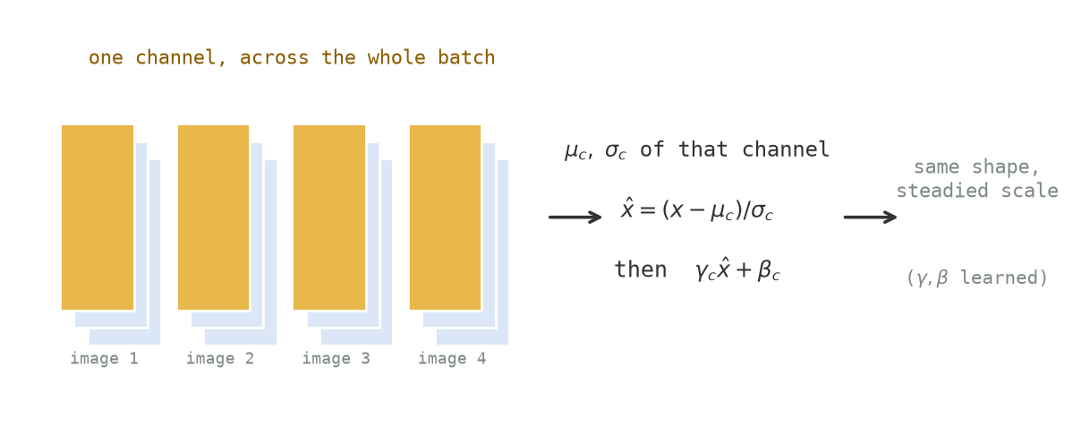
What it improves is conditioning. Each layer now trains against inputs of steady scale, whatever the layers below are doing, so gradients stay usable, learning rates can be set around ten times higher, and initialisation stops being delicate. The original paper explained this as removing “internal covariate shift”; later analysis attributes the benefit to a smoother optimisation landscape [6]. The explanation is still contested; the effect is not.
Two side effects matter in practice. Because each example’s normalisation depends on whichever examples share its batch, BN injects a little noise, which regularises, and networks using it mostly dropped dropout. And because at test time there is no batch, the layer switches to running averages of mean and variance collected during training. That switch is what model.eval() performs. Forgetting it normalises single test images against themselves, which degrades accuracy without raising an error.
BN’s dependence on the batch is also its weakness: at batch size 2 the statistics are noise. GroupNorm and LayerNorm normalise without the batch; LayerNorm’s real entrance is with the transformer (Chapter 8).
3.2.3 The degradation problem
With BN in place, very deep plain networks do train: the gradients flow and the losses descend. They are still worse. He et al. trained a 20-layer and a 56-layer plain network on CIFAR-10 and found the deeper one had higher error on the training set [7]. Read the curves the way Chapter 2 taught: not overfitting — an overfitted network wins on training data and loses on validation; this one loses on both. Figure 3.3 reproduces the experiment with this book’s own runs.
The result contradicts a simple argument. The 56-layer network contains the 20-layer one: set 36 layers to the identity and it could match its shallower sibling exactly. It does not, which says the failure is not capacity but optimisation — nothing steers three dozen layers of freshly initialised weights towards do nothing, because in a plain stack the identity is not a nearby function. It is a specific, delicate configuration of millions of parameters, and gradient descent never finds it.
3.2.4 Residual connections
The repair is one addition sign. A residual block computes
\[ y = F(x) + x, \]
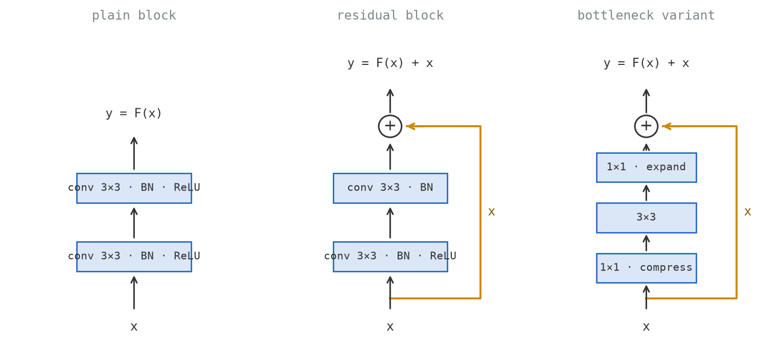
where \(F\) is two or three conv-BN-ReLU layers and \(x\) rides past them on an unmodified skip connection. The block no longer produces the output; it produces the change to the input, and the change defaults to zero. Where a plain stack must construct the identity, a residual stack starts there: push \(F\)’s weights towards zero, which is where weight decay pushes anyway, and the block reduces to its input. An unhelpful block can therefore be neutralised without being removed. It still holds parameters and still costs computation and activation memory; what it no longer costs is accuracy.
The backward pass explains the training curves. Differentiating \(y = F(x) + x\) gives \(\partial L/\partial x = \partial L/\partial y \,(1 + F'(x))\). That constant 1 is a term of the gradient reaching the block’s input untouched by any weight, at every block. The long product that opened this section now has an additive bypass running its whole length, and the vanishing argument no longer applies to the network, only to the optional detours.
ResNets are the template of Chapter 2 built from these blocks, VGG’s design rule kept (\(3 \times 3\) kernels, double channels on downsample), GAP head, BN throughout [7]. Figure 3.4 draws the plain block, the residual block, and the bottleneck side by side. The deeper family members swap in that bottleneck block: \(1 \times 1\) down to a quarter of the channels, \(3 \times 3\) in the narrow space, \(1 \times 1\) back up, at 70,016 parameters where two plain \(3 \times 3\) layers at 256 channels would cost 1,180,160. A single 152-layer version reaches 4.49% top-5 on the validation set, and the six-model ensemble that won ImageNet 2015 reached 3.57% on the test set [7], under the ~5% human estimate. Rerun with skips, the degradation experiment inverts: within this family, deeper is now reliably better, and the follow-up trains past a thousand layers [8]. Depth had been a research obstacle for thirty years; with residual connections it became a design parameter.
Interactive: watch the gradient die
A deep stack at random initialisation, one backward pass, the gradient’s size plotted per layer. Set fifty sigmoid layers with naive initialisation and predict the shape before running — then fix it three ways, one toggle at a time, and rank the fixes. Which survives depth 200 alone?
3.3 Efficiency: MobileNet and EfficientNet in brief
ResNet settled accuracy; the next constraint was everything else. A model that runs on a phone, a robot, or a free Colab GPU is measured on three costs at once, parameters, FLOPs and latency, so an architecture is a point on a frontier of accuracy against cost rather than a single accuracy number.
MobileNet [9] is the separable factorisation of Chapter 2 applied wall to wall: every \(3 \times 3\) dense convolution becomes depthwise-plus-pointwise, the 8.7× saving compounding through the stack, and the whole ImageNet network lands near 4 million parameters. That is a thirtieth of VGG-16’s 138 million, for 70.6% top-1 against VGG’s 71.6% — a point of accuracy given up for a factor of thirty in size. Two multipliers scale it down further, one thinning every layer and one shrinking the input, tracing a family of models along the frontier rather than one point on it.
EfficientNet [10] made the frontier itself the object. Depth, width, and resolution all raise accuracy with diminishing returns, and the paper’s experiments show that scaling one alone saturates sooner than scaling all three together. Its compound rule grows them in fixed ratio, and the resulting family took over the frontier: B0 matches ResNet-50’s accuracy at roughly a tenth of the operations and a fifth of the parameters.
Figure 3.5 plots the chapter on one set of axes. The question an architecture answers stopped being how accurate and became how accurate at what cost, which is the form a deployment decision takes.
3.4 Transfer learning and fine-tuning
3.4.1 Whose features are they?
Chapter 2’s closing question has an empirical answer, and it arrived almost immediately. In 2014 two groups took the penultimate activations of an ImageNet-trained network, the 4096 numbers before the classifier, computed by weights fitted only to ImageNet. One group used AlexNet’s, the other OverFeat’s. They froze those activations and fed them to simple classifiers on entirely different problems: birds, scenes, flowers, furniture [11], [12]. The frozen features beat the hand-crafted state of the art on nearly every benchmark tried. Razavian et al. said it in their title: an astounding baseline. So the features were not narrowly ImageNet’s. A thousand nouns and 1.2 million photographs had been varied enough that most of the network’s layers learned representations useful well beyond that label set, with only the last layers specific to the thousand nouns. Figure 3.6 draws the manoeuvre that observation licenses.
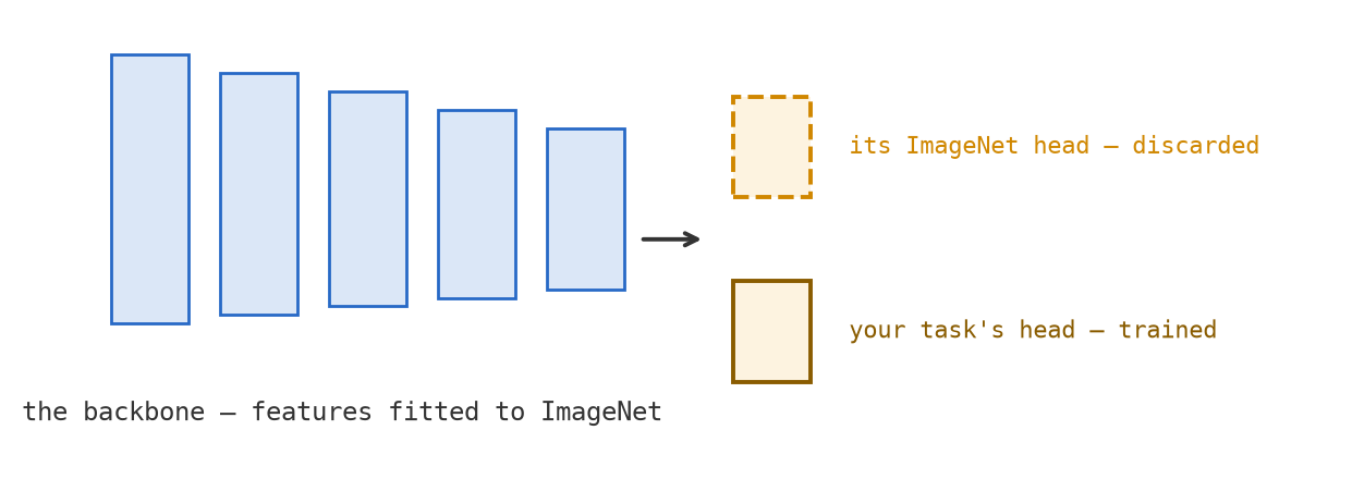
That observation changed practice. If the features transfer, nobody needs to train them twice — and the expensive, data-hungry part of every new vision problem is already done, by someone else, once.
3.4.2 What transfers, by depth
Not all layers transfer equally, and the pattern follows the feature hierarchy of Chapter 2. Yosinski et al. spliced networks at each depth and measured the damage [13]: first-layer features transferred with almost no loss across their task split, and transferability fell off with depth until the last layers, which were specific to the source task. Their experiment used two halves of ImageNet, so the finding is about tasks of that kind rather than about any target domain whatever. The practical reading: early layers are the most reusable, late layers the least, and how much to keep depends on how far the new task sits from the pretraining.
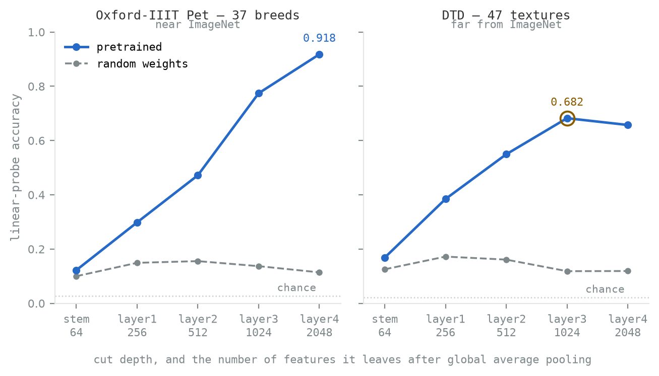
Figure 3.7 runs that experiment on the two datasets Lab 3 uses. Cut a frozen ResNet-50 at five depths, average whatever comes out over space, and fit one linear layer to it: on cats and dogs the accuracy climbs all the way to the last block, while on textures it peaks a block earlier and then falls. The dashed line is the control that makes the rest of the figure mean anything — the same architecture with random weights, probed identically.
figures/runs/train_transfer.py).
3.4.3 The recipes
Using a pretrained backbone comes down to one decision, how much of it to let move, with three standard settings.
A linear probe freezes everything and trains one linear layer on the features. Cheapest, least adjustable, and diagnostically the most honest: whatever accuracy it reaches is credited to the representation alone, which is why probing returns as the standard measuring instrument for self-supervised methods (Chapter 11). A frozen backbone with a new multi-layer head adjusts a little more. Full fine-tuning unfreezes everything and continues training on the new task — almost always at a learning rate around ten times lower than training from scratch, because the pretrained weights are a good solution you are trying to nudge, not noise you are trying to replace, and Chapter 2 said what an oversized step does to a good solution.
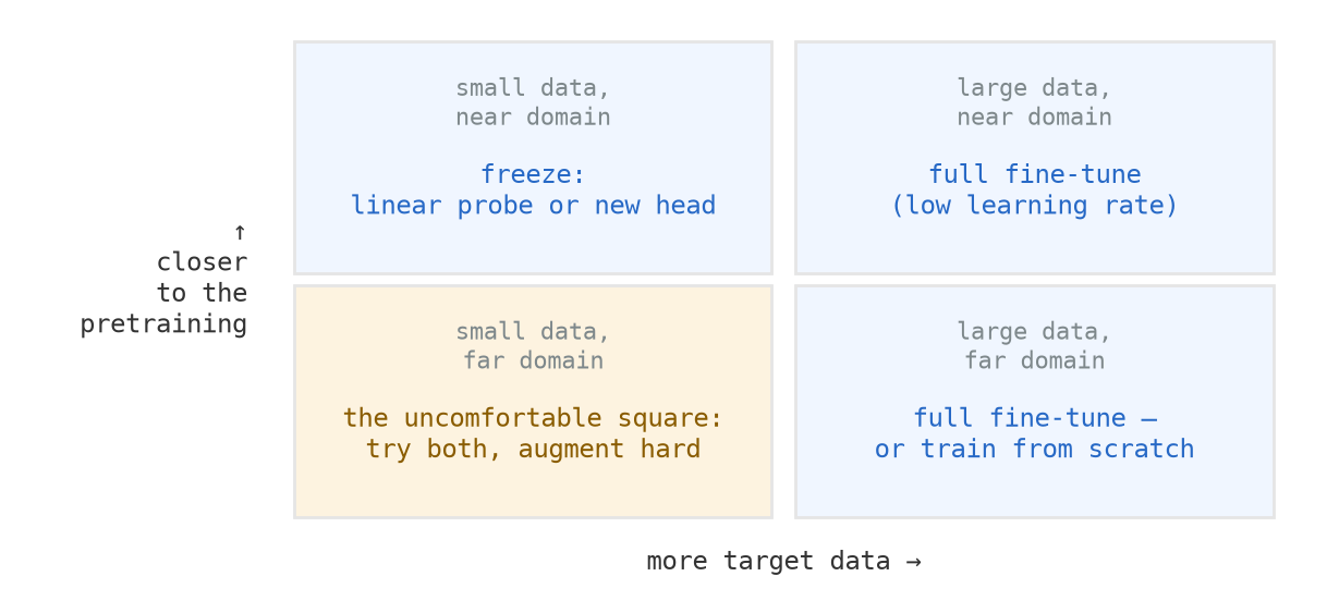
Which setting wins is mostly two questions: how much target data, and how far from the pretraining domain. Small dataset, similar domain: freeze. The probe or frozen head uses the features as they are and cannot overfit much. Large dataset, any domain: fine-tune fully, since there is enough signal to improve even the general layers. Small dataset, distant domain is the uncomfortable square, where freezing keeps features that half-fit and tuning overfits, and the honest answer is try both and augment hard. The boundaries are soft, and they sit at a particular place for a particular problem: on the 37 breeds of Lab 3’s dataset, freezing leads by 6.1 points at one image per class and full fine-tuning has taken the lead by twenty-five, which is a few hundred images either side of the crossing. Lab 3 puts you in that comparison directly — frozen against full fine-tune on the same data, both runs logged. Figure 3.8 lays the choice out.
Three practicalities catch people. Preprocess with the pretraining statistics, because a backbone trained on ImageNet-normalised inputs expects the same at fine-tuning time. Replace the head to match your classes before anything else moves. And when fine-tuning with small batches, freeze BN’s running statistics, for the reason the section above gave: batch statistics from a batch of four are noise.
When transfer fails, it fails by domain gap. X-rays, aerial tiles, and spectrograms are far enough from photographs that the late layers contribute little, and for genuinely large target datasets even the early layers stop paying: given enough data and training time, a network trained from scratch catches up [14]. Pretraining gives faster convergence and better accuracy on small datasets, not a permanent advantage.
Interactive: freeze or fine-tune?
The recipe table’s data axis, run as an experiment. Both recipes start from the same pretrained ResNet-50 on the same 37 breeds, under the same training budget; only the number of training images changes. Commit to an answer before you look: at one image per class, 37 images in total, which recipe wins and by how much? Then find the size at which the answer changes.
Transfer learning inherits the source distribution. What did ImageNet pretraining bake into the features you just reused? The taxonomy, for one: WordNet’s, with person-categories so troubling that the maintainers later removed them. Measurable perceptual habits, for another. ImageNet-trained CNNs tend to classify by texture where humans classify by shape, so that a cat rendered with elephant skin is read as an elephant [15], and your fine-tuned model starts from that prior. And the collection itself was scraped without consent, the history Chapter 1’s provenance reading traced [16]. A pretrained backbone is a dependency like any other: audit what ships inside it.
3.5 The backbone era
This chapter built a noun the rest of the book relies on. A backbone is a pretrained feature extractor, canonically ResNet-50, kept frozen or gently tuned as the first component of a larger system. Every architecture in Part II begins “take a pretrained backbone”; detection, segmentation, and their descendants are structurally elaborate heads. That answers most of the ceiling Chapter 1 closed on: the features adapt to the task, and usually you download them rather than train them. It does not answer all of it, since the transfer holds only as far as the domain gap allows.
One assumption is still standing. Everything here rested on 1.2 million labels, produced by years of annotation. Whether the labels were ever necessary, and whether the images alone could have taught the same features, is the question of Chapter 11.
Exercises
- The ladder’s arithmetic. Using Chapter 2’s parameter formula: verify that VGG-16’s conv1 block (two \(3 \times 3\) layers, 3 → 64 → 64 channels) holds 38,720 parameters while its first dense layer holds 102,764,544; then explain, in two sentences and one computation, how GoogLeNet reaches ~7M parameters total while being deeper than VGG.
- Receptive field per parameter. For 64-in, 64-out channels, compare one \(7 \times 7\) layer against three stacked \(3 \times 3\) layers: receptive field, parameter count, and number of ReLUs. State one thing the single \(7 \times 7\) layer can compute that the stack cannot.
- Batch norm by hand. A channel’s values across a batch of four are \((2, 4, 4, 6)\). Compute the normalised values — take the variance with divisor \(4\), not \(3\), and use no \(\epsilon\) term — then the layer output for learned \(\gamma = 2\), \(\beta = 1\). Now the same input arrives at test time with running mean 3 and running variance 1 — compute the output, and name the bug that produces the training-time answer at test time.
- The gradient highway. Differentiate \(y = F(x) + x\) to show the input gradient contains a term independent of \(F\)’s weights. Explain in one sentence why stacking 100 such blocks does not reintroduce the vanishing product of Section 3.2.1.
- Separability at network scale. A MobileNet-style layer, 512 in, 512 out, \(3 \times 3\): compute dense and separable parameter counts and the ratio. As \(C_{\text{out}}\) grows with \(k\) fixed at 3, what does the saving approach, and why does the pointwise term dominate?
- Choosing the recipe. Four situations: (a) 800 labelled photos of local birds; (b) 400,000 labelled product photos; (c) 600 chest X-rays; (d) 90,000 aerial tiles. For each: probe, frozen backbone, or full fine-tune; the learning rate you would start from relative to from-scratch; and your single biggest concern, one sentence each.
- Audit the inheritance. Design a two-experiment probe of your own fine-tuned model for texture bias in the style of Geirhos et al. [15]: state the stimuli, the measurement, and the result that would convince you the bias transferred.
Lab 3
Lab 3: fine-tune a pretrained ResNet-50 on a small custom dataset; frozen backbone vs full fine-tune — log both runs and compare their curves; visualise your augmented batches before training on them.

Further reading
- Simonyan and Zisserman [3] — VGG; the ablation tables are the argument.
- Szegedy et al. [4] — GoogLeNet; read for how the parameter count is controlled.
- Ioffe and Szegedy [5], and Santurkar et al. [6] — batch norm, and the later argument about why it works.
- He et al. [7] — ResNet; the degradation experiment in section 4 repays close reading.
- Howard et al. [9] and Tan and Le [10] — the efficiency frontier, built and then formalised.
- Yosinski et al. [13] — what transfers, measured layer by layer.
- Geirhos et al. [15] — texture bias; the stimuli alone are worth the visit.
- He, Girshick, and Dollár [14] — the honest counterweight: when pretraining does not help.
References
The paper also hangs two auxiliary classifiers off the middle of the network, extra losses meant to push gradient into the early layers — a scaffold that batch normalisation, below, made unnecessary.↩︎