7 Recurrent Networks and Sequence Modelling
Course week 7.
Chapter 6 showed how a network can produce a prediction at every image location. Some visual tasks require a different kind of output. An image caption is a sequence of words whose length varies, and choosing each word requires information from both the image and the caption produced so far.
This chapter develops recurrent networks, which process a sequence by updating a running state. We use a simple copying task to follow how a network reads and generates sequences, examine how it learns across many steps, and then apply the same ideas to translation and image captioning.
7.1 Sequence modelling
A sequence is an ordered collection of elements, such as the frames of a video or the words of a caption. Order matters: rearranging the frames changes the action we see, and rearranging words can change a sentence’s meaning. Sequence lengths may also vary. A video may contain many frames or only a few; an image caption may need three words or fifteen.
Sequence tasks differ in their inputs and outputs. Video classification maps many frames to one label, while image captioning maps one image to many words. Frame labelling produces one output for each input frame; translation produces an output sequence that may differ in length and word order. Figure 7.1 places these arrangements side by side.
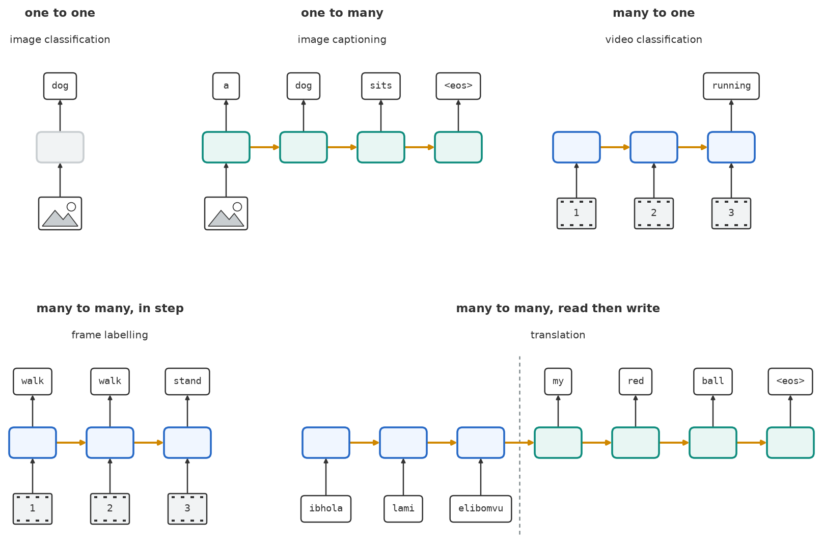
Two arrangements are central to this chapter. Captioning is a one-to-many task: an image provides the visual input, and the network generates words one at a time until it emits a stop symbol. Translation maps one sequence to another, often producing a sequence of a different length, and corresponding words need not appear in matching positions. We will examine an encoder–decoder arrangement that reads the full input before generating its output. To make the flow of information easier to follow, we use a simpler task: copying a short string of digits. For this copying task, we require the model to finish reading before it begins writing, so it has to retain the information needed to reproduce the string.
7.2 Recurrence
A recurrent neural network (RNN) processes a sequence by updating a hidden state. At each step, it combines the next input with the previous state to produce a new state. This state is a fixed-length vector that learns to summarise information relevant to the task. Its size stays the same as more inputs are read.
The operation that updates the state is called a recurrent cell. The same cell uses the same learned parameters at every timestep. Longer sequences therefore require more computation, but no additional parameters.
Let \(x_t\) represent the input at step \(t\), and \(h_{t-1}\) the previous hidden state. The update is
\[ h_t=f_W(x_t,h_{t-1}), \]
where \(W\) denotes the cell’s learned parameters. The first step uses an initial state \(h_0\), often set to zero. The state carries information between steps of one sequence; for a new, independent sequence, the encoder starts again from its initial state. A simple recurrent cell computes
\[ h_t=\tanh(W_xx_t+W_hh_{t-1}+b). \]
Here, \(W_x\) is the learned input-to-hidden weight matrix, \(W_h\) is the learned hidden-to-hidden weight matrix, and \(b\) is the learned bias vector. The two matrix products map the current input and the previous state into the hidden-state space; adding the bias and applying \(\tanh\) element-wise produces the updated representation. These parameters are shared across all timesteps.
Consider the digit string 4 2 7. Each symbol is converted into an embedding: a vector retrieved from a learned table. The cell reads the embedding of 4 and updates its state, then reads 2 alongside that state, and finally reads 7. Drawing these steps side by side is called unrolling the network. The drawing shows several copies of the cell, all using the same parameters.
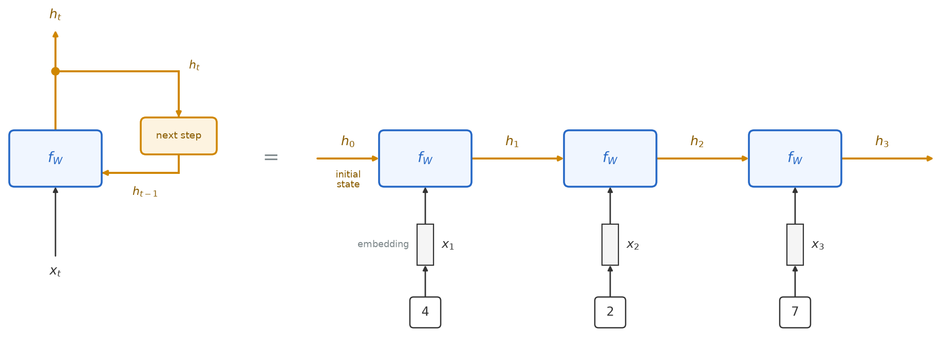
This resembles the weight sharing of a convolution, but the dependency differs. A convolution can process its positions in parallel because their inputs already exist. A recurrent cell must wait for the preceding state before computing the next one.
For our copying task, reading is followed by writing. An encoder reads the input sequence, and its final hidden state initialises a separate recurrent decoder. In this arrangement, the final encoder state is the decoder’s only direct access to the input sequence.
At each decoder step, an output layer converts the hidden state into scores for the possible symbols, and a softmax turns those scores into probabilities. A special start symbol, <sos>, supplies the first input. During generation, each selected symbol becomes the next step’s input, and the decoder stops when it selects <eos>. The desired output for our example is therefore 4 2 7 <eos>.
During training, we can supply the correct preceding symbol instead of the decoder’s own prediction. This is called teacher forcing. The model must still predict the next symbol, and cross-entropy measures its error at each output step. Because the input to the next step can differ from the decoder’s own choice, the hidden states that follow differ too.
For 4 2 7, the training inputs are <sos> 4 2 7, and the corresponding targets are 4 2 7 <eos>. Even if the decoder predicts the first digit incorrectly, its next training input is the correct digit 4.
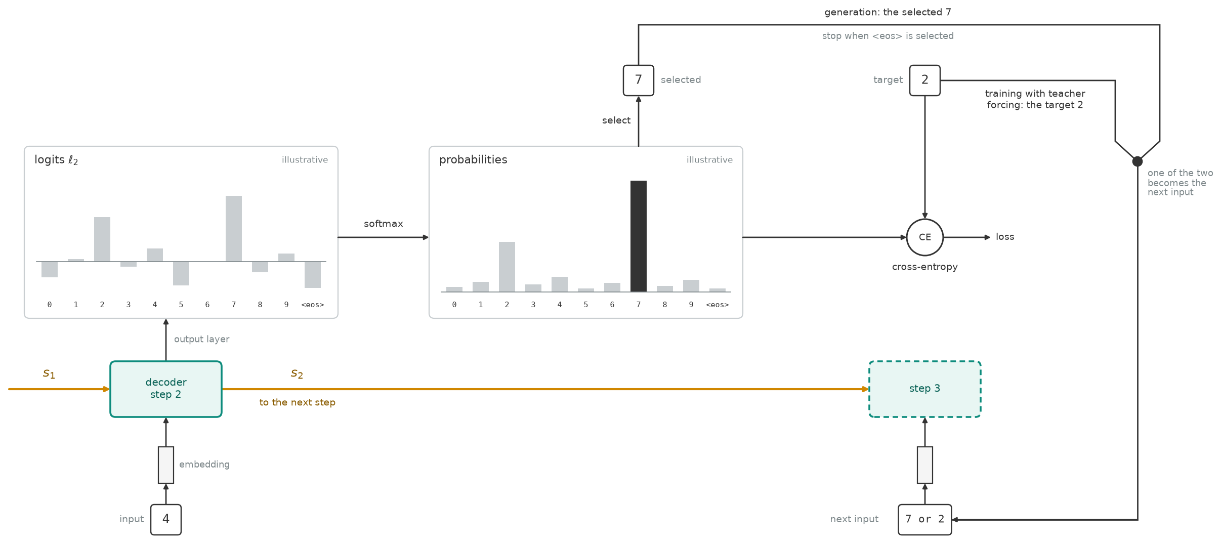
The encoder and decoder each reuse their own parameters across steps; they need not share parameters with one another. Figure 7.4 animates the complete read-then-write process and the state connecting its two halves.
<sos> and feeds each symbol it writes back in as its next input until it writes <eos>. Step through it and note where the decoder could last receive information about the input.
7.3 Learning across recurrent steps
7.3.1 Backpropagation through time
An error at the end of a sequence may depend on information read near the beginning. In our copying task, an incorrect output digit may reflect how the encoder represented that digit, how subsequent updates changed the state, or how the decoder used the final summary. Training must assign responsibility across these operations.
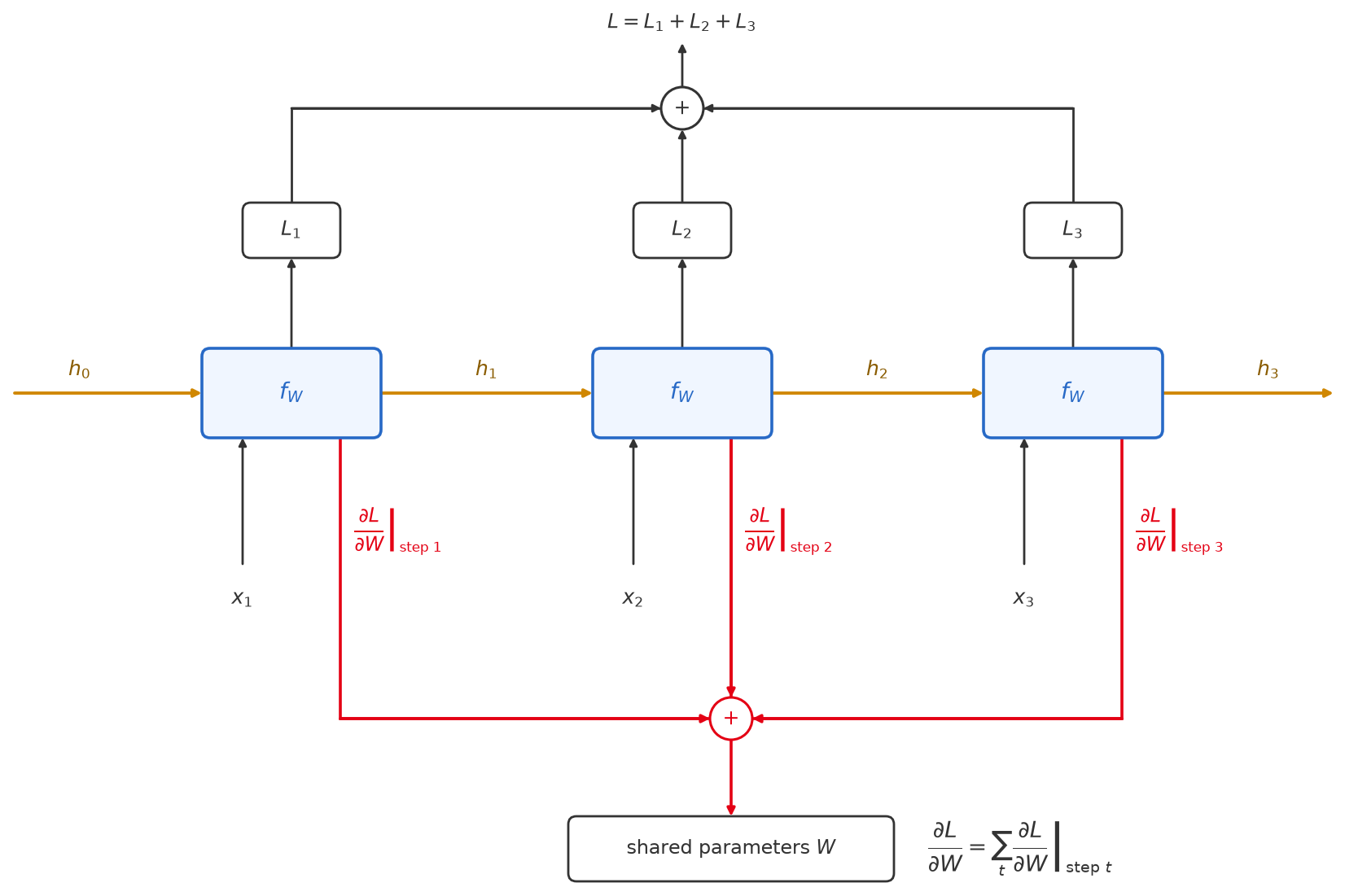
Backpropagation through time applies ordinary backpropagation to the unrolled network. Starting from the output losses, the chain rule carries gradients backwards through the decoder and into the encoder. Each application of the recurrent cell contributes to the gradient of its shared parameters; these contributions are added before the parameters are updated (Section D.2). Figure 7.5 shows this for three steps with a loss at each: every step sends its own contribution to the single set of parameters \(W\), and the update uses their sum.
7.3.2 Vanishing and exploding gradients
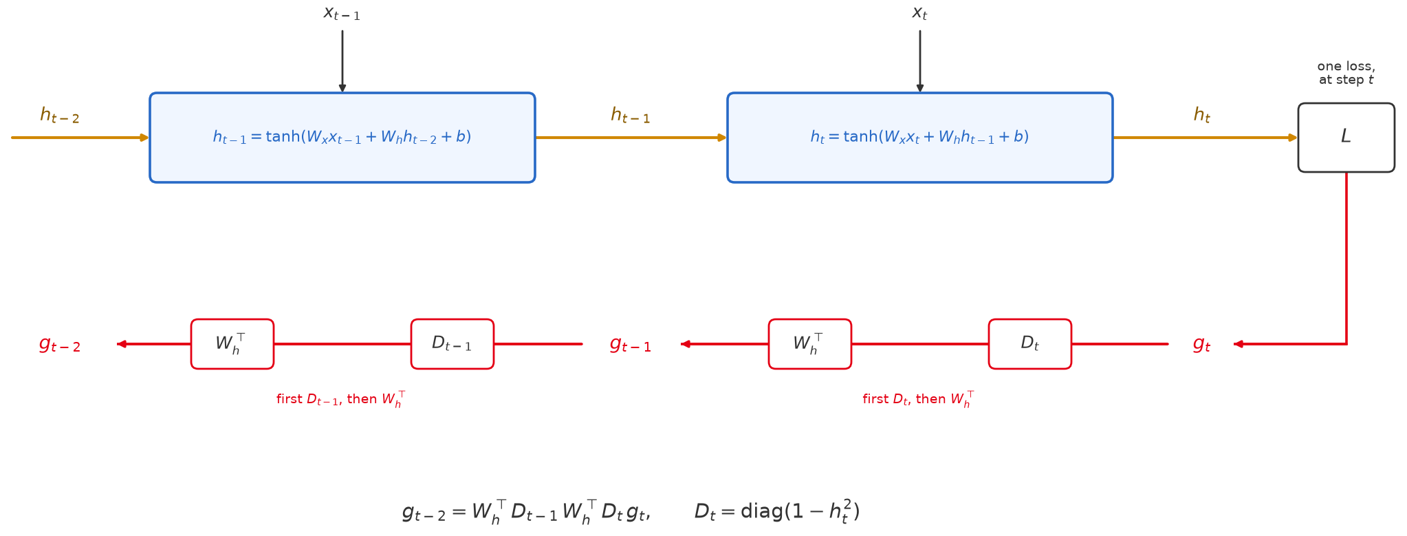
For a loss at a later step, let \(g_t=\partial L/\partial h_t\) be the gradient arriving at hidden state \(h_t\). For the simple tanh cell above, one step backwards gives
\[ g_{t-1}=W_h^\top\left[(1-h_t^2)\odot g_t\right]. \]
Here, \(\odot\) means element-wise multiplication, and \(1-h_t^2\) is the element-wise derivative of tanh. Writing \(D_t=\operatorname{diag}(1-h_t^2)\) for the diagonal matrix of these derivatives, the step is \(g_{t-1}=W_h^\top D_t\,g_t\), the form Figure 7.6 uses. Each backward step therefore applies \(W_h^\top\) again, together with that step’s activation derivatives. For a linear recurrence, with no tanh, start from a loss at the final step \(T\). The repeated multiplication is especially clear:
\[ \begin{aligned} g_{T-1} &= W_h^\top g_T,\\ g_{T-2} &= W_h^\top g_{T-1} = (W_h^\top)^2 g_T,\\ g_{T-3} &= W_h^\top g_{T-2} = (W_h^\top)^3 g_T,\\ &\vdots\\ g_{T-k} &= (W_h^\top)^k g_T. \end{aligned} \]
The nonlinear cell includes the activation derivatives between these matrix multiplications. It is their combined effect that determines whether the gradient shrinks or grows. Losses at several output steps contribute additional gradient terms, but each follows the same backward rule.
Backpropagating through many recurrent steps involves repeatedly multiplying gradients by the derivatives of the state updates. When these transformations repeatedly shrink the signal, contributions from distant steps can become very small, producing a vanishing gradient. The network then receives little guidance on how to change an early state to improve a much later prediction.
When the transformations repeatedly amplify the signal, the gradient can instead become very large: an exploding gradient. This can lead to unstable parameter updates. Both are learning difficulties across many steps, even when a useful representation could in principle fit into the state.
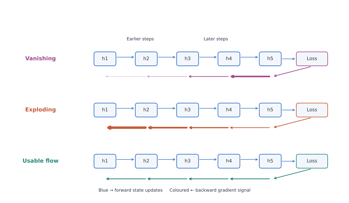
Gradient clipping helps control exploding gradients by rescaling the combined gradient when its norm exceeds a chosen threshold. It limits unusually large updates, but does not restore a learning signal that has already vanished.
7.3.3 Gated memory: LSTMs and GRUs
Long short-term memory (LSTM) networks and gated recurrent units (GRUs) modify the state update to make information easier to retain across many steps [1], [2]. They use learned gates—values between zero and one—to control how much information is carried forward or replaced. The gates depend on the current input and previous state, allowing the network to learn when to preserve information and when to update it.
An LSTM carries a separate cell state \(c_t\) alongside its hidden state \(h_t\). Three learned gates control how memory is retained, updated and exposed:
- The forget gate, \(f_t\), scales the previous cell state. A value near one retains that component; a value near zero removes it.
- The input gate, \(i_t\), controls how much candidate information is written into the cell state.
- The output gate, \(o_t\), controls how much of the transformed cell state contributes to the hidden state.
Each gate is a vector, computed by applying a sigmoid to a learned combination of the current input \(x_t\) and previous hidden state \(h_{t-1}\). Its components therefore lie between zero and one. A separate tanh transformation produces the candidate memory \(\tilde{c}_t\). The cell update is
\[ c_t=\underbrace{f_t\odot c_{t-1}}_{\text{retained memory}}+\underbrace{i_t\odot\tilde{c}_t}_{\text{new information}}, \qquad h_t=o_t\odot\tanh(c_t). \]
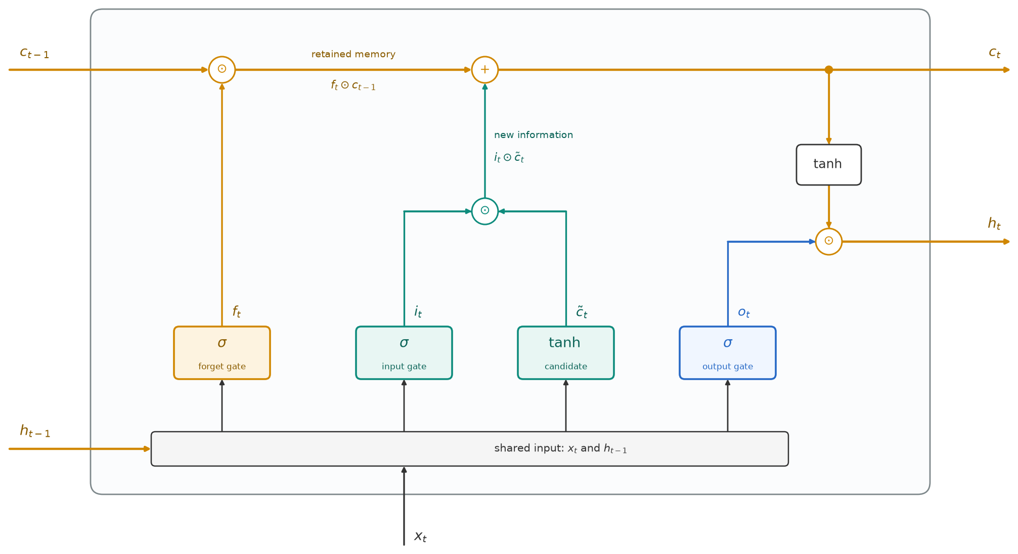
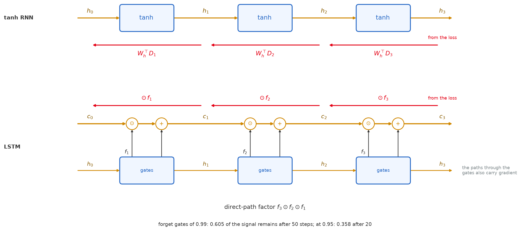
Here, \(\odot\) means element-wise multiplication. If the forget gate is near one and the input gate near zero, the cell can carry its previous memory forward with little change. Along this direct memory path, the backward gradient is scaled by the forget gate rather than repeatedly multiplied by the recurrent weight matrix. Figure 7.9 compares this route with the tanh RNN’s; other gradient paths pass through the gates themselves.
A GRU uses a single hidden state. Its update gate controls the mixture of the previous state and a candidate replacement, while its reset gate controls how much of the previous state contributes to that candidate [2]. Writing the update and reset gates as \(z_t\) and \(r_t\), respectively,
\[ \tilde{h}_t=\tanh\!\left(W_xx_t+W_h(r_t\odot h_{t-1})+b\right), \qquad h_t=\underbrace{z_t\odot h_{t-1}}_{\text{retained state}}+\underbrace{(1-z_t)\odot\tilde{h}_t}_{\text{new information}}. \]
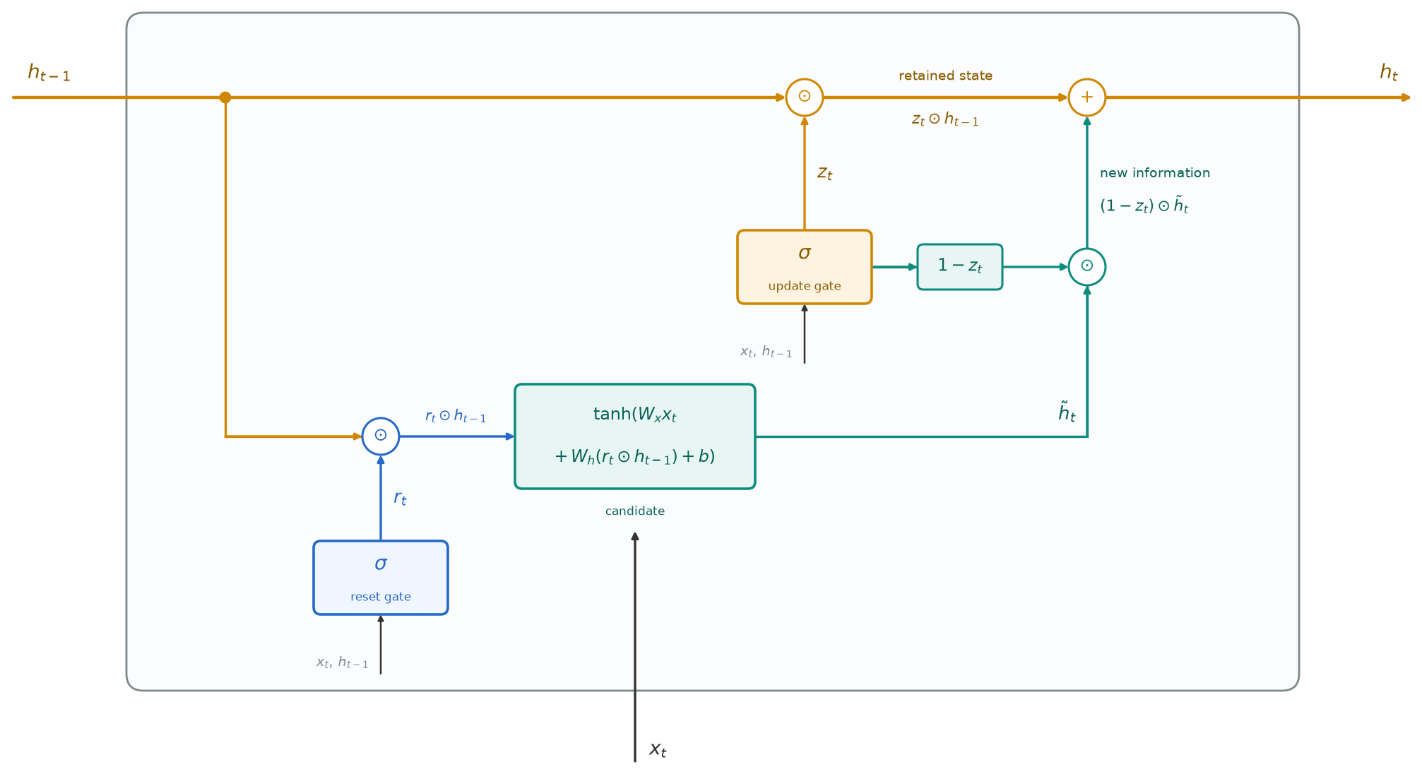
The gates are sigmoid outputs computed from the current input and previous hidden state; \(W_x\), \(W_h\) and \(b\) are learned parameters. In this convention, an update gate near one keeps the previous state, while a value near zero favours the candidate. A reset gate near zero reduces the previous state’s influence on that candidate.
Both designs provide paths that can preserve information and support gradient flow. They make long dependencies easier to learn, but do not guarantee stable gradients or perfect memory. Appendix D develops the gate equations and gradient behaviour.
Gated cells can serve as the encoder and decoder in the copying model above. The same arrangement also supports tasks in which the output describes or transforms the input.
7.4 Translation and image captioning
7.4.1 Machine translation
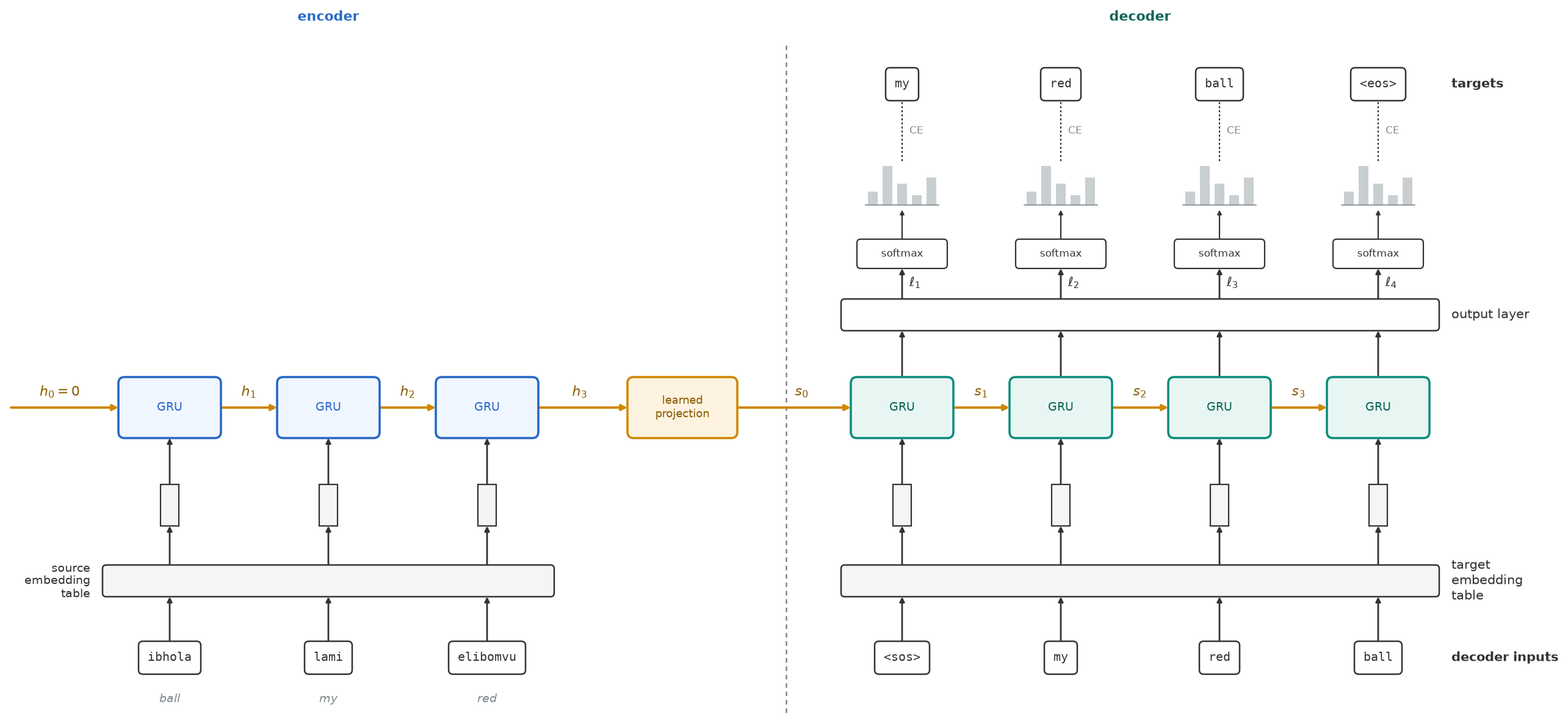
In machine translation, a recurrent encoder reads a sentence in one language, and a recurrent decoder generates a sentence in another [3]. The training data consists of paired source sentences and their translations. Each sentence is split into tokens—words or pieces of words—which are represented by integer IDs and then looked up in an embedding table. The source and target languages can have different vocabularies and separate embedding tables.
To make the data flow concrete, consider a single-layer GRU encoder and decoder. The encoder starts from a zero hidden state and reads the source embeddings in order. After the last source token, its final state summarises the sentence. A learned projection maps that state into the decoder’s initial hidden state; its output width must match the decoder’s hidden-state width. We write the decoder’s states as \(s_t\), starting from \(s_0\), to keep them apart from the encoder’s \(h_t\). The encoder and decoder have separate learned parameters.
The decoder first receives the embedding of <sos>. It combines that embedding with \(s_0\) to compute its next hidden state, \(s_1\), then a linear output layer produces one score, or logit, for each token in the target vocabulary. Softmax turns these scores into probabilities. The state is carried to the next recurrent step, while the next token is supplied through the embedding table. These are two distinct inputs: the state carries the accumulated information, and the token says what was just written.
For the isiZulu source ibhola lami elibomvu, a target translation is my red ball. We treat each written word as one token in this example. With teacher forcing, the decoder inputs are <sos> my red ball, and the targets are my red ball <eos>. Cross-entropy is evaluated against the next target token at each step, including the end token. Its gradient passes back through the decoder, the projection and the encoder, so the source representation is learned for the translation task. For batches with padded target sequences, padding positions are excluded from the loss. A padded source must likewise use the encoder state after its last real token, rather than after the padding.
At inference, the target translation is unavailable. We can use greedy decoding: select the highest-probability token, feed its embedding into the next step, and continue until <eos> is selected. A maximum output length also prevents a model that has not learned to stop from generating indefinitely. The output can have a different length and word order from the source; in this example, ibhola (“ball”) precedes lami (“my”) and elibomvu (“red”), while English places “my” and “red” before “ball”.
7.4.2 Image captioning
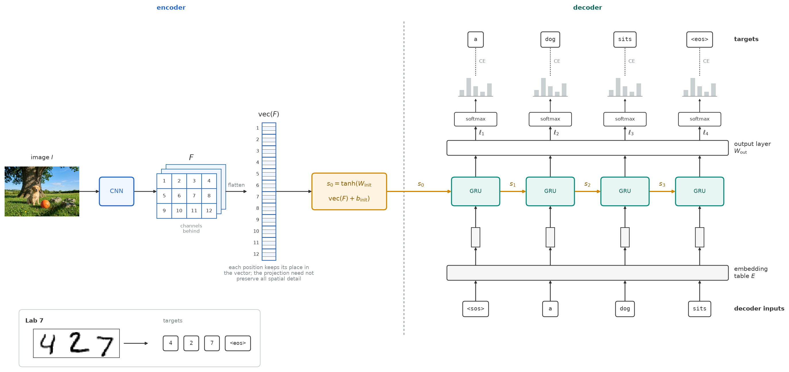
Image captioning uses the same encoder–decoder pattern with an image as the input. Training pairs consist of an image and a caption describing it. A CNN computes visual features, and a recurrent decoder predicts the caption tokens. Show and Tell combines a CNN with an LSTM decoder [4]. It supplies the image representation as an input once, before the word inputs; the recurrent state then carries visual information as the caption is generated.
A simple variant projects the CNN’s features directly into a GRU’s initial hidden state. Let \(I\) be the image and \(F\) its CNN feature map. Flatten the feature map into a vector, then apply a learned linear map and tanh:
\[ F=\operatorname{CNN}(I),\qquad s_0=\tanh\!\left(W_{\mathrm{init}}\operatorname{vec}(F)+b_{\mathrm{init}}\right). \]
Here, \(\operatorname{vec}\) flattens the feature map by listing its values in a fixed order. Features from different image locations occupy different entries in the vector, so the learned projection can give different weights to features on the left and on the right. It combines these entries into an initial hidden state of the width required by the GRU. This implementation uses a fixed image size so that the projection always receives the same number of inputs.
The decoder now follows the same process as in translation. If \(y_{t-1}\) is the preceding token and \(E\) is the learned embedding table, one step is
\[ s_t=\operatorname{GRU}\!\left(E[y_{t-1}],s_{t-1}\right),\qquad \ell_t=W_{\mathrm{out}}s_t+b_{\mathrm{out}}. \]
The vector \(\ell_t\) contains the next-token logits. The initial token is <sos>; subsequent inputs are correct preceding tokens during teacher forcing and selected predictions during generation. The embedding table, GRU and output layer are reused at every step. During training, cross-entropy sends gradients through the output layer and recurrent steps back into the image projection and CNN. If the loss implementation accepts logits and includes softmax internally, pass \(\ell_t\) directly rather than applying softmax first.
The same architecture can read a row of handwritten digits: the CNN encodes the image, and the GRU generates the digits in order from left to right. An image of 4 2 7 uses decoder inputs <sos> 4 2 7 and targets 4 2 7 <eos>. Each digit is a vocabulary symbol with a learned embedding. Place the images on a fixed-size canvas, padding shorter rows with blank space. Separately, pad target sequences when assembling a batch, exclude those padding positions from the loss, and keep the end token as a genuine prediction target. At inference, show the image and generate the digits without supplying the correct string. Lab 7 develops this example into a complete image-to-sequence recogniser.
Both applications connect an input representation to a sequence generator. Translation uses a recurrent encoder to read a sentence; captioning uses a convolutional encoder to read an image. The recurrent decoder turns that representation into an output one step at a time. We now have the components needed to read a sequence, maintain a learned state and generate a new sequence from it.
The next chapter, Chapter 8, examines what information the decoder can access and how that access can change during generation.
Exercises
- What does each task read and write? For each task, say what the network reads, what it writes, and whether the output has one element for each input step: (a) assigning one action label to a video clip; (b) labelling every frame of a video as “walking” or “standing”; (c) writing a caption for a photograph; (d) translating a sentence from English into isiZulu; (e) reading the digits from an image of a handwritten postcode. Which tasks naturally support an output at each input step? How would the others use the read-then-write arrangement introduced in this chapter?
- Counting parameters. A simple recurrent cell reads 32-dimensional embeddings and keeps a 64-dimensional hidden state. Count the parameters in \(W_x\), \(W_h\) and \(b\). How does the count change if the input string has 1,000 digits rather than 10? Add an output layer that scores eleven symbols, the ten digits and
<eos>. Optional extension: Use the chapter’s LSTM and GRU equations, with one input matrix, one recurrent matrix and one bias for each gate or candidate, to count the parameters of an LSTM cell and a GRU cell of the same sizes. - One update at a time. A recurrent cell with a scalar state computes \(h_t=\tanh(0.5\,x_t+0.8\,h_{t-1})\), starting from \(h_0=0\). Each digit enters as \(x_t=\text{digit}/10\). Compute \(h_1\), \(h_2\) and \(h_3\) for the string
4 2 7, then for7 2 4. The two strings contain the same digits. Explain why their final states differ, and what that implies about how the state represents order. - Training with the answer in hand. The target string is
3 1 4 1. Under teacher forcing, write the decoder’s input and target at each step, including<sos>and<eos>. Suppose the decoder assigns probabilities 0.6, 0.3, 0.8, 0.5 and 0.9 to the correct symbol at the five steps. Compute the cross-entropy at each step and the mean over the sequence. At inference, the decoder predicts7instead of1at the second step. What does it receive as input at the third step, and why might training with teacher forcing leave it unprepared for that input? - Repeated multiplication. In a linear recurrence with a scalar state, \(h_t=w\,h_{t-1}+u\,x_t\), the gradient reaching \(h_{T-k}\) is \(w^k\) times the gradient at \(h_T\). Compute this factor for \(w=0.9\) and \(w=1.1\), at \(k=20\) and \(k=50\). Now add a tanh, set \(w=1.2\), and suppose every state along the path has the value 0.5, so that each step also contributes the derivative \(1-0.5^2\). Compute the factor after 20 steps. What does the result say about judging gradient behaviour from the recurrent weight alone?
- Clipping a gradient. A combined gradient is \((3,4,12)\), and gradients are clipped to a norm of 5. Compute the clipped gradient and show that its direction is unchanged. Explain why clipping can prevent a destructive update, but cannot help when the gradient reaching early steps has already become very small.
- How long does an LSTM remember? One component of an LSTM’s cell state holds the value 1.0. For the next ten steps, the input gate is zero in that component. What fraction of the value remains if the forget gate is 0.9 at every step? What if it is 0.99? Describe the gate values that would erase the component and write a candidate value of 0.6 in a single step. Finally, relate the product of forget gates to the gradient along the direct cell-state path.
- The GRU’s two gates. In one component, \(h_{t-1}=1.0\) and the candidate is \(\tilde{h}_t=-0.5\). Using the chapter’s convention, compute \(h_t\) for update gates \(z_t=0.9\) and \(z_t=0.2\). Then explain what a reset gate near zero changes: which quantity it affects, and how that differs from the effect of a small update gate.
- Where the input goes. Draw the encoder–decoder that copies
4 2 7, and the image-captioning model from this chapter. On each, mark what the decoder receives about the input, and at which step. What difficulties might arise when copying longer strings while the hidden-state size stays fixed? Distinguish a model trained on these lengths from one tested on strings much longer than those seen during training. - An image of any width. The image encoder in this chapter flattens a CNN feature map and projects it into the decoder’s initial hidden state. Why does this require a fixed image width? Design an alternative encoder for rows of handwritten digits whose images have a fixed height but varying widths. It should use the same learned parameters for every width, preserve the left-to-right order, and supply a fixed-size initial state to the decoder. Do not resize every image to the same width or assume a maximum width for padding. Sketch your design using components from this chapter and explain how information flows through it. Which parts grow with image width, and which stay fixed? Would accepting wider images necessarily mean reading longer digit strings accurately?
Lab 7
Lab 7: an image-to-sequence recogniser that reads strips of handwritten digits, with a CNN encoder and a GRU decoder trained with teacher forcing, scored by exact-string accuracy and character error rate; then longer strings than it was trained on.

Further reading
- Hochreiter and Schmidhuber [1] — the LSTM cell and its approach to retaining information across recurrent steps.
- Cho et al. [2] — gated recurrent units in an encoder–decoder for translation.
- Sutskever et al. [3] — sequence-to-sequence learning with recurrent encoders and decoders.
- Vinyals et al. [4] — combining a CNN image encoder with a recurrent caption generator.
- Pascanu et al. [5] — vanishing and exploding gradients, and gradient clipping.