2  Learning the Filters: CNNs

NoteLearning objectives

• Explain why learned filters became dominant in computer vision, and what changed in 2012
• Assemble convolution, nonlinearity, and pooling into a CNN, and reason about shapes, parameter counts, and receptive fields
• Distinguish the dilated, transposed, grouped, and separable convolutions, and say what question each one answers
• Train a CNN end to end (loss, stochastic gradient descent, backpropagation, regularisation) and read the training curves
• Recognise a CNN’s first layer as a learned filter bank

Skills ladder. W&B from this week onward: every run logged, every config recorded. Seed everything. And the overfit-a-single-batch ritual: before any real training run, overfit one fixed batch to 100% accuracy and a very small loss.

Chapter 1 combined hand-designed filters and descriptors with components learned from data, including the visual vocabulary and classifier. CNNs move the learning further down the pipeline: the filter weights and intermediate representations are trained jointly with the classifier. The architecture, training data, loss, and hyperparameters are still chosen by people, but the parameters within the model are fitted by one error signal propagated through the network.

2.1 From MR8 to AlexNet’s first layer

In the ImageNet challenge, an entry looks at a photograph and names what is in it, choosing among 1,000 classes. Because many photographs contain several plausible answers, the challenge’s headline score is top-5 error: the entry proposes five classes, and is wrong only if the true label is not among them. Figure 2.1 shows what the four extra guesses are for.

Figure 2.1: What the challenge asks. Four photographs and the five classes a trained AlexNet scores highest for each. The first two are outright hits, though the retriever wins by only nine points over bloodhound. The cat’s label sits third, behind two classes describing much the same animal, tiger cat and Egyptian cat; the Shih Tzu’s also sits third, behind Dandie Dinmont and the near-identical Lhasa apso. The difficulty is in fine distinctions of this kind: 118 of the 1,000 classes are dog breeds. Top-1 error would score the last two photographs as failures; top-5 does not. Photographs CC0 via Wikimedia Commons; predictions from torchvision’s AlexNet on the \(224 \times 224\) centre crop shown.

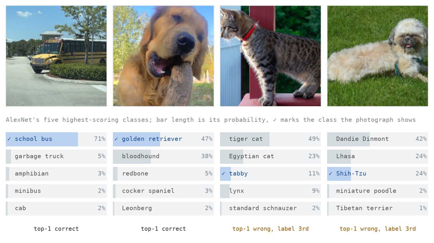
The winning 2011 classification entry had a top-5 error of 25.8%. In 2012, the AlexNet-based SuperVision submission achieved 16.4% using the provided training data; an ensemble that included networks pretrained on the larger ImageNet 2011 release reached 15.3%. The best non-CNN entry recorded 26.2% [1], [2]. By 2013, almost all classification entries used deep convolutional networks.

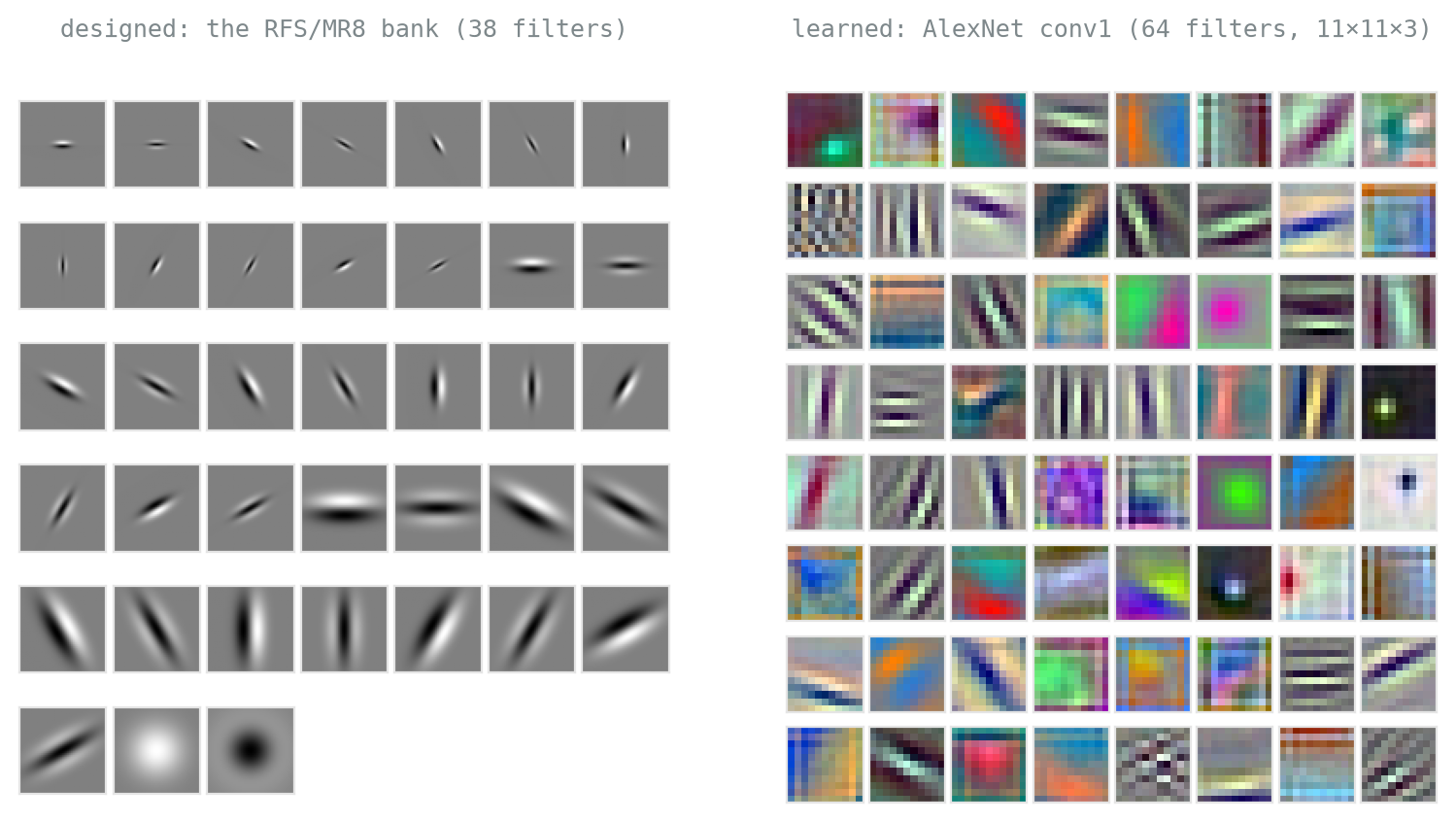
Original AlexNet’s first convolutional layer contains 96 filters of size \(11 \times 11 \times 3\). Each can be displayed as an RGB patch. Many are selective for orientation or spatial frequency; others respond to colour contrasts or blobs. Their weights were not specified by hand but were fitted for ImageNet classification. They resemble some classical filters, but they do not reproduce the MR8 bank. Deeper layers learn combinations of these responses over wider receptive fields. Figure 2.2 compares the two banks.

Figure 2.2: The hand-designed and learned banks. Left: the 38 filters in the RFS/MR8 bank of Section 1.7. Right: the 64 first-layer filters in torchvision’s pretrained AlexNet. Their weights were fitted on ImageNet; many are orientation-, frequency-, or colour-selective. Colour-opponent filters were already familiar from biological and classical vision, so their appearance is a correspondence rather than a new filter family. The original AlexNet used 96 first-layer filters; the torchvision architecture shown here is a later variant.

Interactive: read the learned bank

Chapter 1 read the kernel before looking at what it does, and the same habit works on filters nobody wrote. Click any of the 64 and its response in the scene appears alongside it, signed, mid-grey for zero, as Section 1.4 displayed Sobel. Pick a tile, predict what it will draw out of the scene, then click it. Then find a filter whose response you cannot explain from its tile.

The idea was not new. Fukushima’s neocognitron used layers of local filters in 1980, trained by a self-organising procedure rather than end-to-end gradient descent [3]. LeCun and colleagues developed gradient-based training for convolutional networks, and by 1998 LeNet-5 formed part of commercial systems for reading handwritten digits on bank cheques [4]. CNNs remained useful for specialised tasks but did not dominate large-scale visual recognition. AlexNet combined several developments: 1.2 million labelled training images, an efficient GPU implementation, ReLU nonlinearities, data augmentation, and dropout [1]. Convolution and backpropagation were established ideas; their combination with this data, hardware, and training procedure produced the 2012 result.

The rest of the chapter takes the network apart. First the layer itself: what a learned filter is, and what shape it has. Then the operations between layers, which set what each filter can see. Then the zoo of convolution variants, and the assembly of the whole network. Training comes last: where the parameters are actually learned.

2.2 The convolution layer

2.2.1 Why not a fully-connected layer?

The obvious way to put an image into a neural network is the way that works for everything else: flatten it to a vector and connect every input to every unit. For a \(224 \times 224\) colour image and a first layer of 1,000 units, that is \(224 \times 224 \times 3 \times 1000\) weights, just over 150 million in the first layer alone. Even at CIFAR’s \(32 \times 32\) (the lab’s scale), one modest dense layer costs three million weights.

The count is not the only problem. A dense layer treats each pixel-channel value as a separate input coordinate, with no built-in preference for nearby pixels or shared detectors across positions. In principle, it can learn local structure from data. In practice, however, it must learn the same pattern separately at each location: seeing an eye in the top-left updates different weights from seeing one elsewhere. Its learned patterns are therefore tied to position, and the layer is not translation equivariant. Its input dimensionality is also fixed: a standard dense layer built for \(224 \times 224\) images cannot directly accept another image size.

Convolution is the dense layer with two constraints: each output reads only a local window, and the same weights are used at every window position. The result is the operation from Chapter 1: a kernel sliding over the image. Weight sharing makes the parameter count independent of the image’s height and width. With stride 1, a shift of the input shifts the feature map in the same way, apart from padding and boundary effects. A convolutional layer can process variable spatial dimensions large enough for its kernel, although later layers may impose a fixed input size. Figure 2.3 imposes the two constraints one at a time, and Lab 2 compares the resulting structure with a dense network on the same task.

Figure 2.3: Two constraints, applied in order. Fully connected: every output unit reads every input via its own weight, and the outputs are never recomputed using the same weight index. Locally connected: each unit reads a window of three, so the connections collapse, but each window still has its own weights and the indices keep climbing. Weight sharing: every window uses the same \(w_1 w_2 w_3\), and the sweep shows them riding along the input rather than advancing. That last picture is a kernel being slid, which is the convolution of Chapter 1 arriving by subtraction rather than by design. Of the three counts at the foot, the first two grow with the input and the third does not.

2.2.2 A filter whose numbers are unknowns

A convolution layer, then, is Chapter 1’s operation with the kernel entries left blank. Sobel’s \([-1, 0, 1]\) columns were an argument about derivatives; the Gaussian’s weights follow from a formula; MR8’s bank was a design. Here the kernel starts as small random numbers and ends wherever training puts it. The habit the kernel zoo taught still applies: read the numbers and you know the filter. Only their source has changed.

Figure 2.4 shows the same thing at its smallest possible scale: nine numbers and one question. The task is the easiest one that still needs a filter: is the bar in this image vertical or horizontal? The only instruction the kernel ever receives is whether the answer came out right. Before running it, write down the nine numbers you would use, then compare them with where training arrives. A positive column with negative flanks is the bar detector of Section 1.7, reached by gradient descent rather than by construction. It is worth pressing new random start a few times: the run that ends with its positive column on the left and the run that ends with it on the right are the same filter twice, and neither was the one anybody had in mind.

Figure 2.4: Nine numbers, fitted. One \(3 \times 3\) kernel slides over a \(9 \times 9\) image holding a single bar; its strongest response anywhere in the image is the score, and the score decides vertical or horizontal. The kernel begins as noise, and the loss curve and the nine traces below it show what the training signal alone does to those numbers: they separate, then settle, into a column of one sign flanked by the other, an oriented bar detector of the family Section 1.7 built by hand. The middle panel shows both images live, with the filter’s best position ringed in gold.

One piece of fine print from Chapter 1 settles itself here. The “convolutions” in deep learning are correlations, with no kernel flip, and here the distinction stops mattering: a learned kernel has no prior orientation to preserve. If the flipped version were useful, training would learn it in that form.

2.2.3 The kernel is a volume

Chapter 1 convolved one grayscale image with one flat kernel. CNNs usually move beyond that setup immediately: a layer applies multiple filters and produces multiple feature maps, so subsequent filters must operate across channels. This is where the shapes change.

Unless stated otherwise, this chapter uses dense convolution, in which every filter reads every input channel. For a colour input, a \(3 \times 3\) filter therefore has size \(3 \times 3 \times 3\): nine weights for red, nine for green, and nine for blue. At each position, the products are summed across space and channels to produce one number. Sliding the filter produces one two-dimensional feature map. Grouped and depthwise convolutions, introduced below, relax the requirement that every filter read every channel.

One filter produces one feature map. A layer stacks the maps from \(C_{\text{out}}\) filters into an output volume with \(C_{\text{out}}\) channels. In the next dense convolution, each filter has \(C_{\text{out}}\) input channels. Its depth therefore matches the number of maps produced by the preceding layer. Figure 2.5 shows one step.

Figure 2.5: One convolution layer, run forwards. The input volume is \(5 \times 5 \times 3\), and the kernel sliding through it is \(3 \times 3 \times 3\), the same depth as the input, because in a dense convolution each filter reads every input channel. Each stop of the sweep sums its products across space and channels and writes one cell of one feature map. Press play: when the gold filter has visited all nine positions, its map is complete, and the second filter, purple with its own 27 weights, sweeps the same input and writes a second map in front of the first. One map per filter is all \(C_{\text{out}}\) means, and the colours mark authorship only; the maps hold response values.

The parameter count follows directly. A layer with \(C_{\text{out}}\) filters of size \(k \times k \times C_{\text{in}}\), each with a bias, holds

\[ k \cdot k \cdot C_{\text{in}} \cdot C_{\text{out}} + C_{\text{out}} \]

parameters. AlexNet’s first layer has 96 filters of \(11 \times 11 \times 3\), so \(11 \cdot 11 \cdot 3 \cdot 96 + 96 = 34{,}944\) parameters. The formula does not contain the image height or width, so the number of learned parameters is the same for a thumbnail and a larger image. The computational cost is not: the filter is evaluated at more positions, so multiply-adds and activation memory grow with the output’s spatial dimensions. In parameter counts, the main term is \(k^2 C_{\text{in}} C_{\text{out}}\), and the product \(C_{\text{in}} C_{\text{out}}\) often dominates once the kernel size is fixed.

Interactive: the kernel with depth

One \(3 \times 3 \times 3\) kernel, one small three-channel input, one step at a time. Before pressing anything: the kernel holds 27 weights and the input is \(5 \times 5 \times 3\), so how many numbers land in the output map? Step through a position and watch the three per-channel products collapse into one, then add the second filter and see where its map goes.

2.2.4 Bias and nonlinearity

Two small additions complete the layer used here. Each filter has a bias, one number added to every position of its map; that is the \(+\,C_{\text{out}}\) in the parameter formula. The biased map then passes through a nonlinearity \(f\), applied to each value independently. Written out, filter \(c\)’s output map is

\[ A_c \;=\; f\bigl(I * K_c + b_c\bigr), \qquad c = 1, \dots, C_{\text{out}}: \]

the convolution of Chapter 1, one number added everywhere, one function applied everywhere. A common choice of \(f\) is the ReLU (rectified linear unit), \(f(v) = \max(0, v)\). Negative responses become zero; positive ones pass unchanged. Earlier networks used smooth S-shaped functions: the sigmoid, and its zero-centred cousin tanh. The reason ReLU displaced them is discussed in Chapter 3. For now it is enough that ReLU is cheap and does not flatten out for large positive inputs. Figure 2.6 draws the three side by side.

Figure 2.6: Three nonlinearities. The sigmoid squashes everything into \((0, 1)\) and flattens at both ends, so large inputs stop mattering; tanh centres the squash on zero but keeps the flat ends; the ReLU passes everything positive through at slope 1, however large. What that difference costs at depth is the opening subject of Chapter 3.

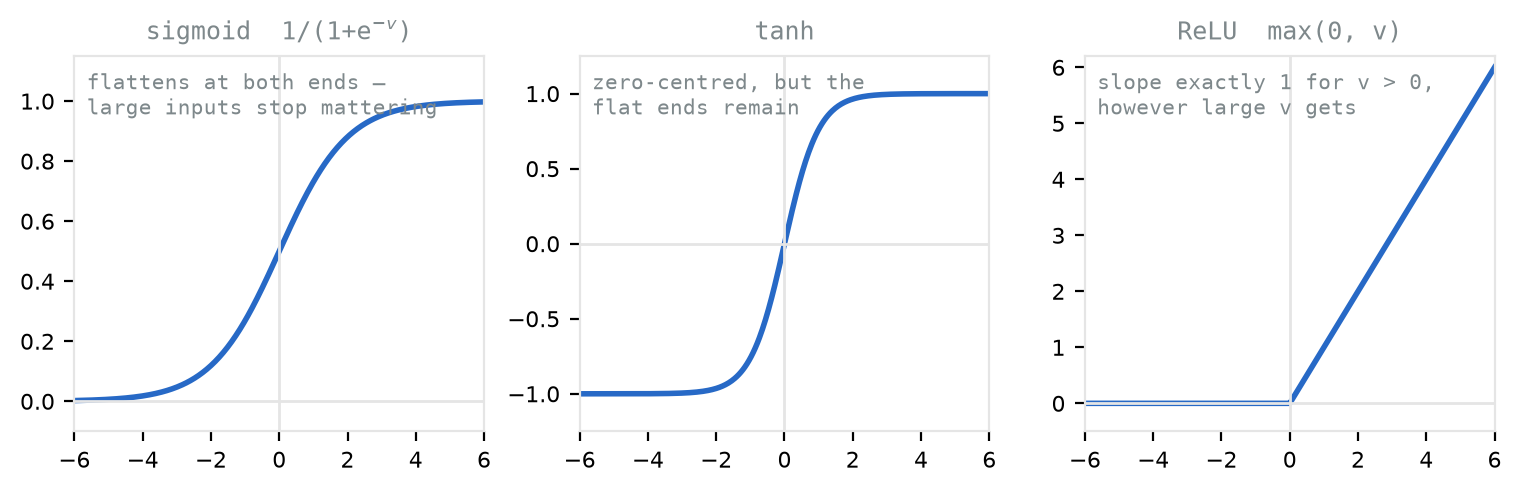
A convolution followed by a bias is an affine operation. A stack of affine convolutional layers with no nonlinearities can be represented by one affine convolution with a larger effective kernel, subject to the same boundary conventions. Extra layers change the parameterisation but do not make the overall function nonlinear. ReLU prevents this collapse: compositions of convolution and ReLU can represent functions that no single convolution can.

2.2.5 The 1×1 convolution

Set \(k = 1\) in the formula and something useful remains. A \(1 \times 1\) convolution has no spatial window, seeing one position at a time, but it still spans all \(C_{\text{in}}\) channels: each filter is a weighted sum across the channels at a point. It is pure channel mixing, with \(C_{\text{in}} \cdot C_{\text{out}} + C_{\text{out}}\) parameters.

You have used one. The grayscale conversion of Section 1.1.4, \(Y = 0.299R + 0.587G + 0.114B\), is a \(1 \times 1 \times 3\) convolution with one filter, the dot product that section flagged with fixed, for now. Now it is neither fixed nor limited to one output: a \(1 \times 1\) layer re-mixes 256 channels into 64, or 64 into 256, wherever a network needs its channel count changed cheaply. That re-mixing is how GoogLeNet and ResNet hold down their parameter counts and multiply-adds (Chapter 3), and it is half of the separable convolution below. Figure 2.7 draws its shape.

Figure 2.7: The \(1 \times 1\) convolution has the shape of a rod through the channels. It covers one position at a time but spans the full input depth, so each stop re-mixes the channels at a given position into a single output value. Press play: the stride-1 layer visits all 25 positions and preserves the input’s height and width. It mixes channels at each position without mixing information between neighbouring positions.

2.3 Pooling, stride, and receptive fields

2.3.1 Shrinking the map

Section 1.5 put the problem plainly: a \(3 \times 3\) kernel sees three pixels across, objects live at every scale, and the answer there was to shrink the image rather than grow the kernel. A CNN faces a related problem: later units need to combine information over wider regions without applying large kernels at full resolution. Pooling and strided convolution shrink intermediate feature maps, allowing receptive fields to grow more quickly while reducing computation.

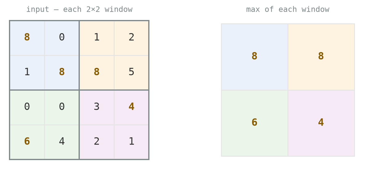
There are two common ways. Pooling summarises each small window of a map and has no parameters; the usual summary is the maximum of a \(2 \times 2\) window taken with stride 2 (max pooling), sometimes the average. Strided convolution folds the shrinking into the layer itself: a stride of 2 computes every second position, typically reducing each spatial dimension by about half while it filters. The exact output size also depends on the input size, kernel, and padding, as the output-size formula of Chapter 1 describes. That formula, and the padding bookkeeping around it, apply here unchanged; exercise 4 of Chapter 1 was practice at this arithmetic. Figure 2.8 shows the operation at its smallest, and Figure 2.9 runs the stride itself.

Figure 2.8: Max pooling, \(2 \times 2\) with stride 2. Each window of four keeps only its largest value (gold); the map halves in each direction, and the layer has no parameters at all.

Figure 2.9: The stride, run live. Pick a stride and press play: gold dots mark the window centres the layer actually computes, grey dots the ones it skips, and the output fills as the kernel lands, drawn at the input’s scale so each output cell is as wide as the stride it stands for. Stride 2 computes a quarter of the positions and halves the map; the output size in the panel is the formula of Chapter 1, evaluated live.

2.3.2 Pooling and translation tolerance

A stride-1 convolution is translation equivariant away from padding and boundaries: shifting the input shifts its feature map. Strided pooling changes that relationship. Its windows are fixed to a sampling grid, so shifting the input by one pixel can move responses between windows and change the pooled values.

Max pooling can nevertheless provide limited translation tolerance. If a strong response moves but remains the maximum within the same pooling window, that pooled value does not change. This depends on the input and the position of the pooling grid; it is not a general invariance guarantee. A shift equal to the pooling stride instead shifts the pooled map by one cell, apart from boundary effects. Repeated downsampling discards spatial precision, which may help classification but is costly for tasks whose output must retain location. Figure 2.10 demonstrates these cases for one feature map.

Figure 2.10: For this feature map, several pooled values survive a one-pixel shift because their maxima remain within the same windows. A two-pixel shift moves the pooled map by one cell, apart from the boundary.

WarningDownsampling can alias

A stride-2 convolution filters its input and evaluates the result on every second spatial position. Its learned kernel could suppress high frequencies, but neither the architecture nor ordinary training requires it to act as a low-pass filter. Max pooling is not a low-pass filter either. Both operations can therefore alias.

After downsampling, a one-pixel input shift changes the sampling phase, so the output need not be a shifted copy of the original output. Translation equivariance then holds only for some shifts and away from boundary effects. Blurring before downsampling improves shift consistency at a small additional computational cost [5].

2.3.3 Receptive fields

A unit in the first layer sees a \(3 \times 3\) patch of the image. A unit in the second layer sees a \(3 \times 3\) patch of feature maps, each position of which already summarises a patch of the image, so its window on the original is wider. Figure 2.11 traces one unit down the stack: it reads nine values, each of those values read nine pixels, and the union of their windows is \(5 \times 5\).

Figure 2.11: One unit, traced back through two layers. The gold unit reads a \(3 \times 3\) window of the map below it. Each value in that window was computed from a \(3 \times 3\) window of its own, and because neighbouring windows overlap, their union on the input is \(5 \times 5\), not \(9 \times 9\). That region is the unit’s receptive field. While subsequent layers use \(3 \times 3\), stride-1 convolutions at this resolution, each further layer widens the field by two pixels.

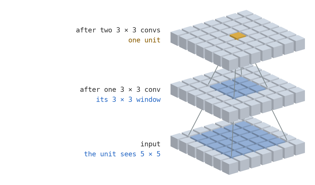
Track the receptive-field size \(R_\ell\) and the jump \(J_\ell\), the distance between neighbouring units measured on the original input. Before the first layer, \(R_0 = J_0 = 1\). For layer \(\ell\), with kernel size \(k_\ell\) and stride \(s_\ell\),

\[ R_\ell = R_{\ell-1} + (k_\ell - 1)J_{\ell-1}, \qquad J_\ell = s_\ell J_{\ell-1}. \]

Both calculations use the values entering the layer. In particular, the kernel samples positions in the preceding map, so receptive-field growth depends on \(J_{\ell-1}\); the new jump \(J_\ell\) applies to the next layer.

For the stack conv \(3 \times 3\), pool \(2 \times 2\)/2, conv \(3 \times 3\), pool \(2 \times 2\)/2, conv \(3 \times 3\), the receptive fields grow through \(3, 4, 8, 10,\) and \(18\) pixels. Applying the same calculation to AlexNet gives a \(163 \times 163\) theoretical receptive field at conv5. Depth is how a \(3 \times 3\) kernel comes to see a dog. Stacking gives later units access to progressively wider regions, while downsampling produces coarser feature maps. This resembles the image pyramid of Section 1.5, but the two are not equivalent: pyramid levels are rescaled versions of an image, whereas CNN layers contain different learned representations. A wider receptive field supplies context; it does not make a standard CNN scale invariant.

The arithmetic gives the field’s outer boundary. Influence within it is not uniform: it falls off roughly as a Gaussian from the centre, so the effective receptive field is considerably smaller than the box [6].

Interactive: receptive fields

Build a stack, then click a unit in its top map. Before clicking, predict the field’s size from the layer list alone; the running arithmetic is displayed, so you can check yourself layer by layer. Then find the cheapest stack whose top units see the whole image, and say whether an extra convolution or an extra pool got you there for fewer parameters. Switching responses on fills the map with a live response from one fixed edge filter standing in for a learned one, and each added stride visibly coarsens it.

2.4 The convolution zoo

Chapter 1’s kernel zoo varied the numbers inside the kernel. This zoo varies the wiring around it. Each variant answers one question about the dense convolution, each is a small change to the arithmetic already on the table, and each is put to work in a named later chapter.

2.4.1 Dilated: a wider view without more weights

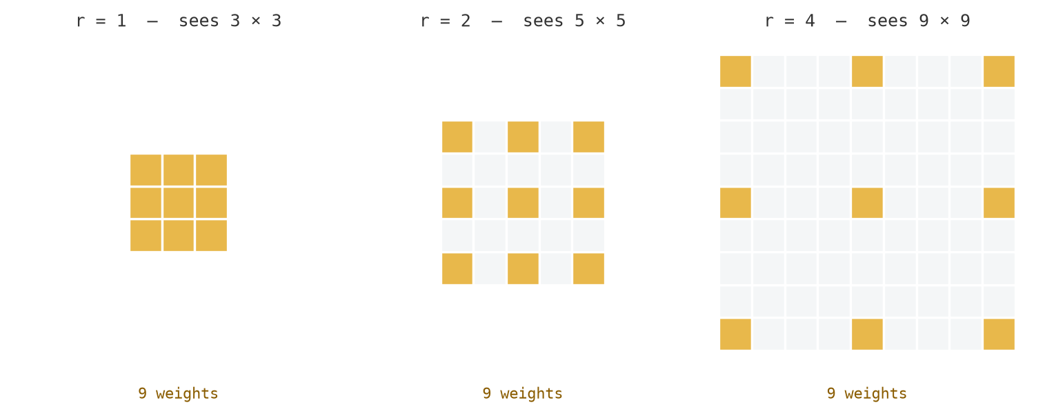
A dilated convolution spaces the weights of a \(k \times k\) kernel \(r\) pixels apart. Its effective size is

\[ k^{\prime} = k + (k-1)(r-1). \]

A \(3 \times 3\) kernel therefore covers a \(5 \times 5\) footprint at rate 2 and a \(9 \times 9\) footprint at rate 4, without adding parameters. With stride 1 and suitable padding, dilation enlarges the receptive field without reducing the map resolution. Rates \(1, 2, 4, \ldots\) make the receptive field grow exponentially with depth. This is useful for dense prediction, where the network needs wide context without further downsampling (Chapter 6). Figure 2.12 shows the spacing.

Figure 2.12: The dilated kernel’s footprint at rates 1, 2, and 4. The nine gold taps are the same nine weights every time; only their spacing grows. With \(k' = k + (k-1)(r-1)\) the footprint runs \(3\), \(5\), \(9\) while the kernel still holds nine spatial weights.

Interactive: dilation arithmetic

The bookkeeping is easier to watch than to read [7]. The widget opens in dilated mode: set the rate, predict the output size with \(k'\) in place of \(k\), then step through and check. Its other modes replay the ordinary arithmetic of Chapter 1 and preview the transposed entry below.

2.4.2 Transposed: getting the resolution back

A strided convolution maps a large grid to a smaller one. A transposed convolution reverses the direction of its connections. Each input value is multiplied by every kernel weight, producing a \(k \times k\) patch that is added to a larger output. The stride sets the spacing between these patches, and overlapping contributions are summed. Its weights are learned like those of any other layer.

The name transposed is literal, and it is the clearest way to see what the operation is. After flattening the arrays, a convolution can be written as \(y = Cx\), where \(C\) is a sparse matrix containing copies of the kernel. A transposed convolution applies \(C^{\mathsf{T}}\). In Figure 2.13 it maps four values to sixteen; it is the transpose of the linear map, not its inverse, and it does not reconstruct the original input.

Figure 2.13: Convolution as one matrix multiply, and its transpose. Top: a \(4 \times 4\) input convolved with a \(3 \times 3\) kernel gives a \(2 \times 2\) output. Left: the same computation as \(y = Cx\), with the input flattened to sixteen numbers and each row of the \(4 \times 16\) matrix \(C\) holding the kernel at one window position. Right: multiplying a four-element vector by \(C^{\mathsf{T}}\) produces a sixteen-element vector, which is the transposed convolution and the origin of its name. The result has the original input shape but does not generally reconstruct the original input.

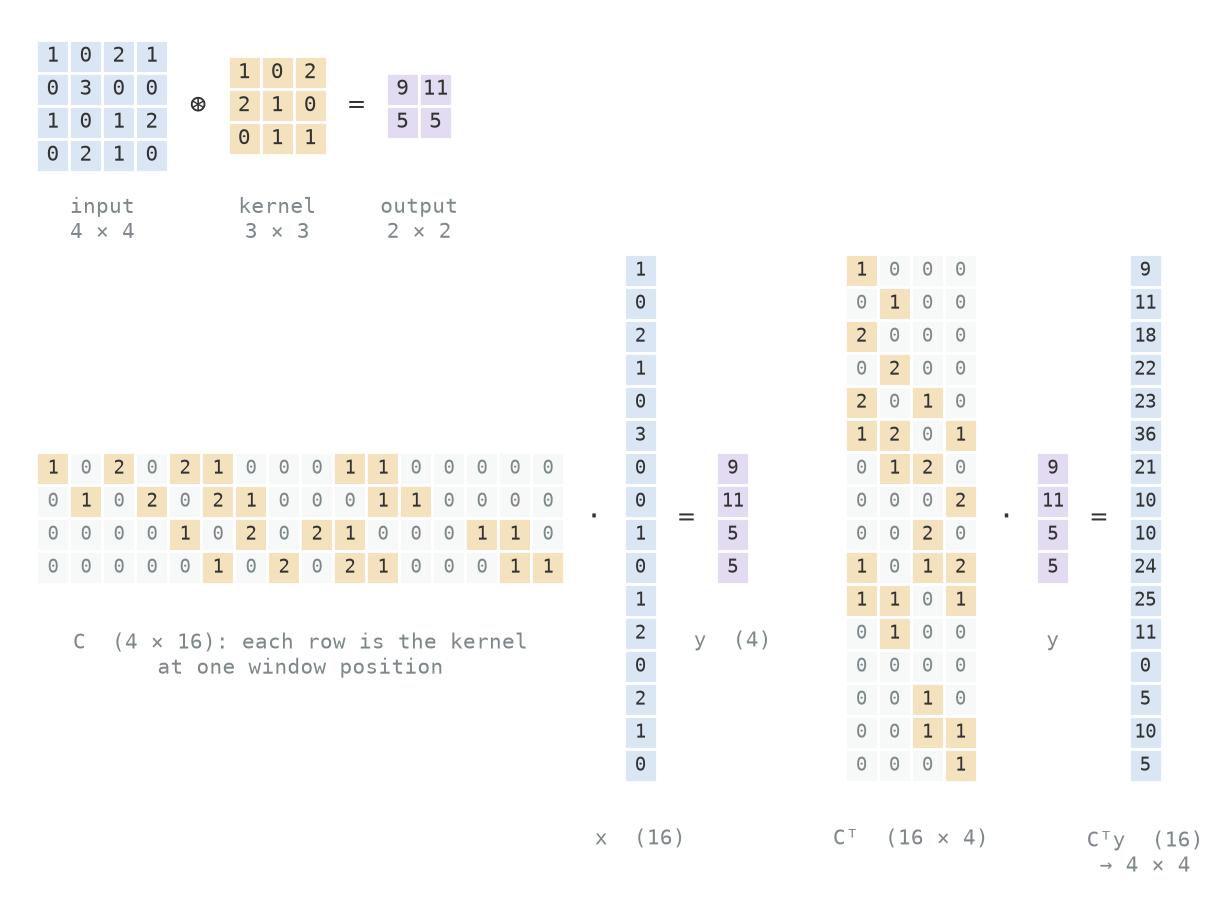
Figure 2.13 uses a particular kernel, and three of its nine weights happen to be zero, which hides part of the pattern. Figure 2.14 draws the same two matrices with the weights left as symbols \(w_{ij}\), so that every slot a weight occupies is visible.

Figure 2.14: The same construction with symbolic weights. Left: \(C\), whose every row holds all nine kernel weights, shifted one window position along each time. Right: \(C^{\mathsf{T}}\), where each of those rows has become a column, so the entries in one row of \(C^{\mathsf{T}}\) are the weights that multiplied that input position in the forward pass. Reading a row of \(C^{\mathsf{T}}\) is reading which weights an input position collects when the operation runs backwards.

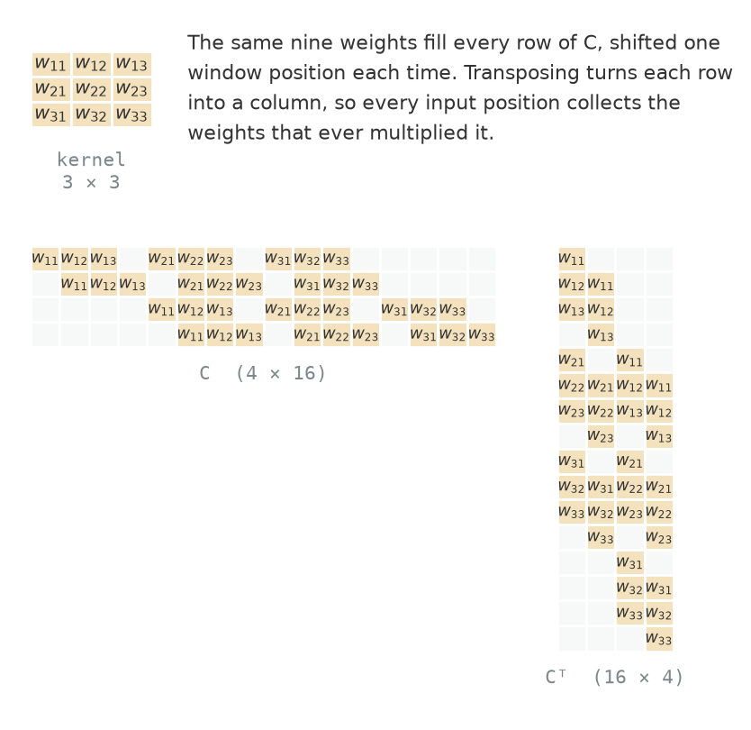
Figure 2.15 runs the arithmetic on real numbers, and shows the second way of computing the same output.

Figure 2.15: The transposed convolution on real numbers, two ways. Deposits: each input value is multiplied by every kernel weight, and the resulting patch is added to the \(5 \times 5\) output. The patches are spaced two positions apart and overlaps are summed. Fractionally strided: a zero between the input samples, padding around them, and an ordinary stride-1 convolution with the kernel rotated \(180°\) give the same output.

For the stride and padding shown, inserting \(s - 1\) zeros between input samples and applying a stride-1 convolution with the corresponding padding gives the same result. The kernel is rotated \(180°\) when the forward operation is implemented as correlation. This construction motivates the name fractionally strided convolution.

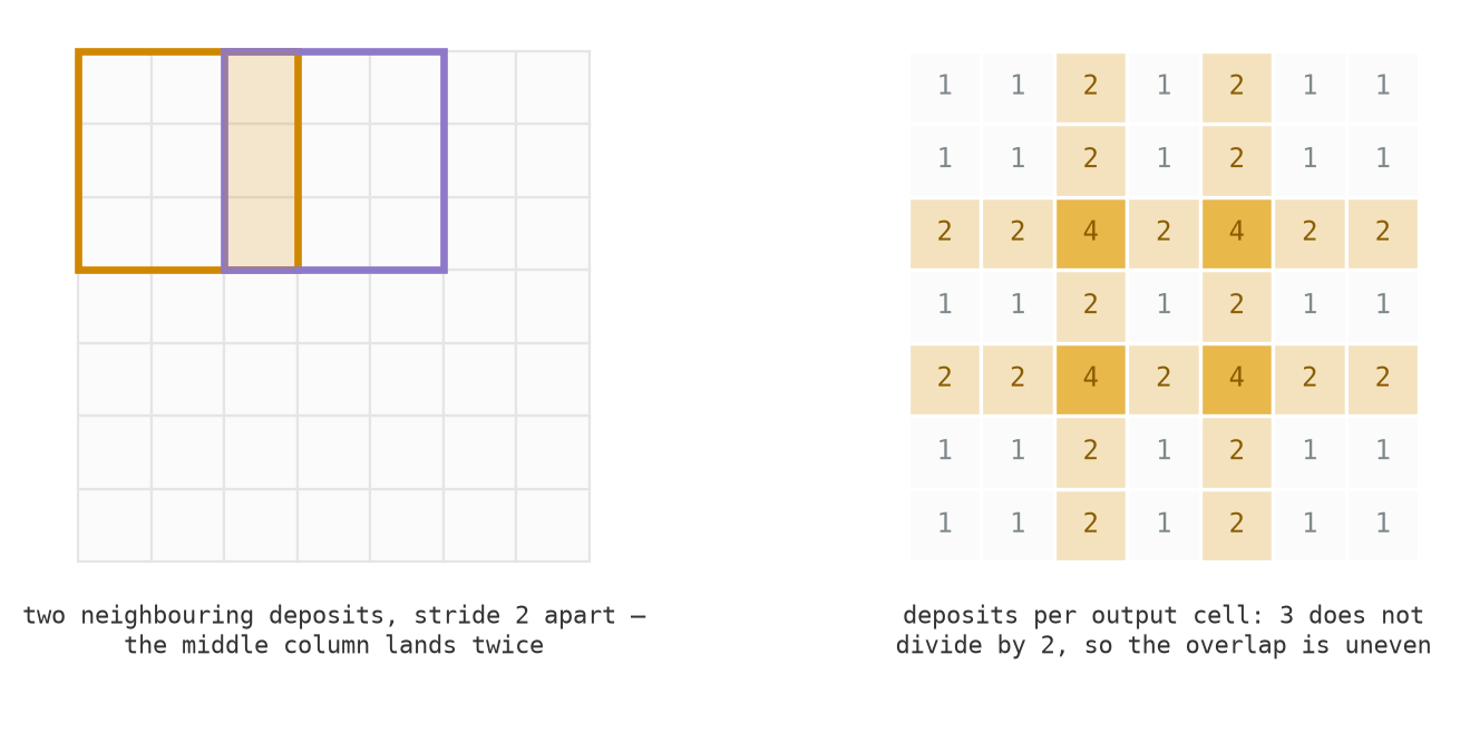
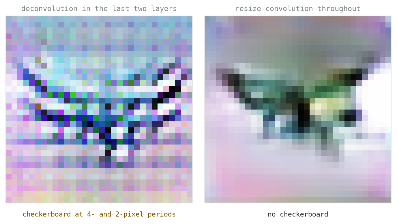
It is sometimes called a “deconvolution”, which it is not: nothing is undone, and the operation is convolution’s shape-transpose. When the kernel size is not divisible by the stride, the patches overlap unevenly, creating a built-in source of checkerboard artefacts [8]. Choosing a divisible kernel size removes this uneven-overlap mechanism, but does not guarantee an artefact-free output. It returns in Chapter 6, where a network that has shrunk its maps must produce a full-resolution answer; the decoder half of U-Net is built from these. Figure 2.16 counts the deposits, and Figure 2.17 shows them surviving all the way into a trained generator’s pictures.

Figure 2.16: Transposed convolution’s deposits: a \(3 \times 3\) kernel at stride 2, from a \(3 \times 3\) input onto its \(7 \times 7\) output. Left: two neighbouring input cells deposit their \(k \times k\) patches two apart, so the middle column lands twice. Right: how many deposits reach each output cell, either 1, 2, or 4, never the same count everywhere, because 2 does not divide 3. That uneven overlap is the checkerboard.

Figure 2.17: The deposit counts, arriving in a generator’s output. Two samples from one GAN, trained twice and differing only in how it upsamples. Left: the last two layers upsample by transposed convolution, and the uneven overlap prints itself over the whole frame, mostly at a four-pixel period contributed by the second-to-last layer, with a weaker two-pixel component from the last. Right: every upsampling step replaced by a nearest-neighbour resize followed by an ordinary convolution, and the pattern is gone. The samples are \(32 \times 32\), shown at 16× with no interpolation; 54% of the left image’s variance lies at periods of four pixels and shorter, against 6% of the right’s. Odena, Dumoulin, and Olah, CC BY 2.0, via Distill.

2.4.3 Grouped: cut the channel product

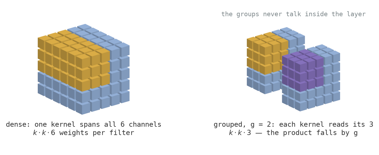
The main term in the parameter count, \(k^2 C_{\text{in}} C_{\text{out}}\), is proportional to the product of the two channel counts, and that product can be cut directly. A grouped convolution splits the channels into \(g\) groups and convolves each group separately: each filter sees only \(C_{\text{in}}/g\) channels, and the parameter count divides by \(g\). The cost is that no information passes between the groups inside the layer.

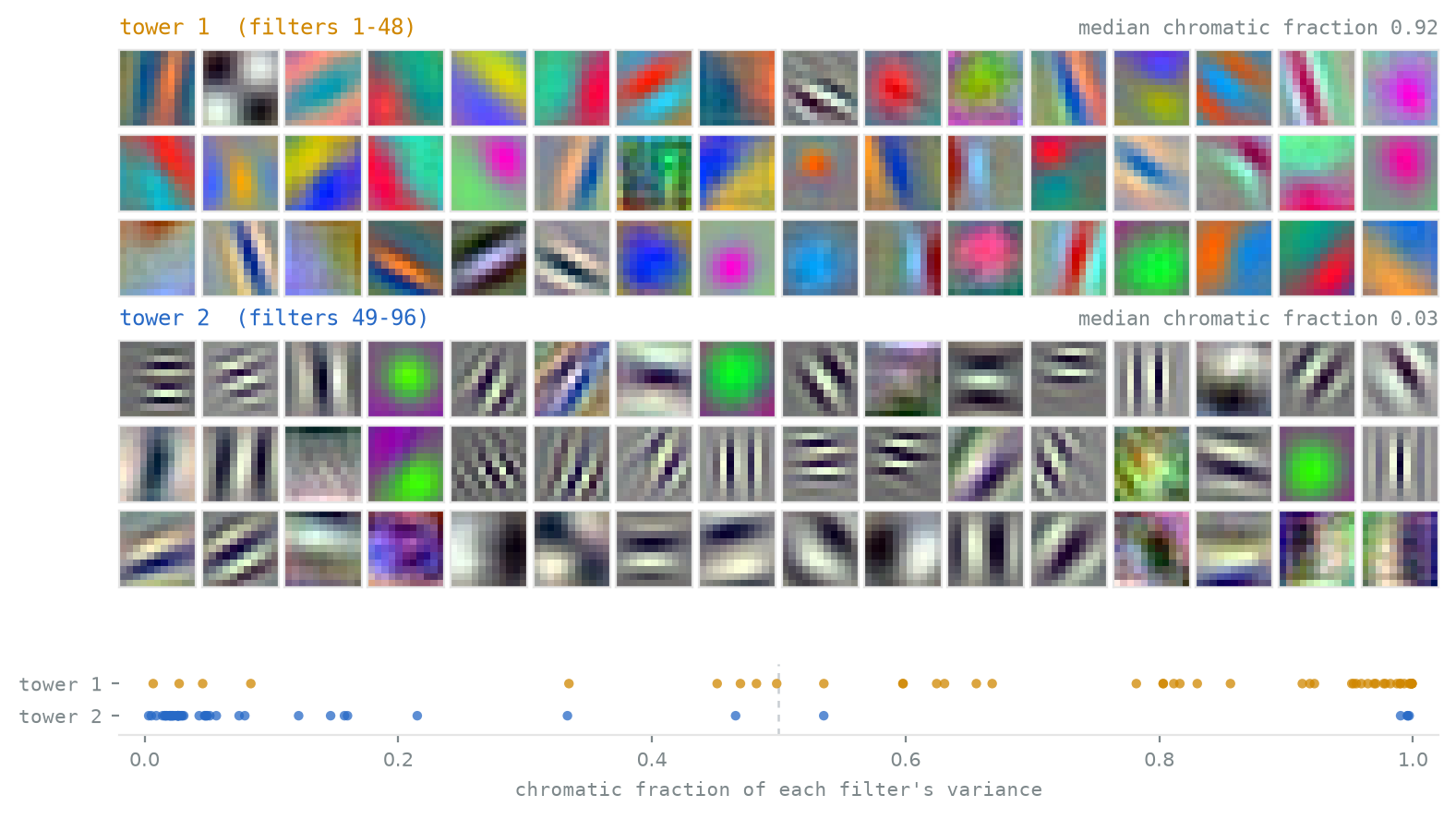
The variant is as old as the revival: AlexNet was grouped out of necessity, its 96 filters split across two 3 GB GPUs that exchanged data only at certain layers. In the original network the two halves specialised, one towards grayscale structure and one towards colour [1]. What began as a hardware workaround returned as a design principle (ResNeXt, [9]). Figure 2.18 compares the wiring, and Figure 2.19 shows the specialisation in a network trained the same way.

Figure 2.18: Dense against grouped wiring, drawn as volumes. Left: one kernel spans all six input channels, \(k \cdot k \cdot 6\) weights per filter. Right: grouped with \(g = 2\); the channels split into two blocks of three, each with its own half-depth kernel, so the weights per filter halve and the two groups exchange nothing inside the layer.

Figure 2.19: The two towers, and what each one learned. All 96 first-layer filters of a grouped AlexNet, drawn in the two halves the architecture separates. One tower has gone to colour and the other to oriented grayscale gratings, which is the specialisation the paper reports. The strip below measures it: for each filter, the share of its variance that survives subtracting its own mean over the three channels, so an achromatic filter sits near 0 and a colour blob near 1. The medians are 0.92 and 0.03. Which tower takes which role is not fixed by the architecture; here the colour half is the first, where the paper’s figure has it second. Rendered from BVLC AlexNet, a replication of the paper’s architecture trained on ILSVRC-2012 and released for unrestricted use via the Caffe model zoo; the split appearing in an independent training run is what makes it a property of the architecture rather than of one run.

2.4.4 Separable: factor the kernel

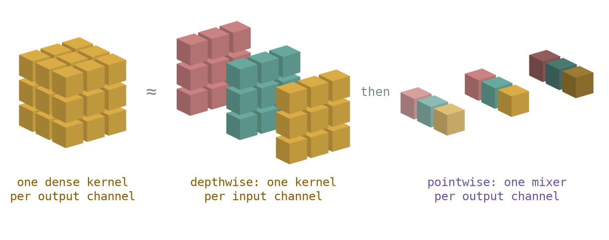
A dense filter’s \(k \cdot k \cdot C_{\text{in}}\) weights do two jobs at once, filtering across space and mixing the channels. A depthwise separable convolution factors a dense convolution into two operations, one for each job. This is analogous to Gaussian separability, but it separates spatial filtering from channel mixing rather than horizontal filtering from vertical filtering. First, a depthwise step applies a \(k \times k\) filter to each input channel independently, and a different filter to each: \(C_{\text{in}}\) kernels of \(k^2\) weights, not one kernel reused. A pointwise \(1 \times 1\) convolution then mixes those \(C_{\text{in}}\) filtered maps to produce \(C_{\text{out}}\) output channels, using a different set of mixing weights for each one. Ignoring biases, the parameter count falls from

\[ k^2 C_{\text{in}}C_{\text{out}} \]

to

\[ k^2 C_{\text{in}} + C_{\text{in}}C_{\text{out}}. \]

For a \(3 \times 3\), 256-to-256 convolution, that is an 8.7× reduction in parameters. MobileNet uses these blocks through most of its convolutional body (Chapter 3). Figure 2.20 shows the factorisation.

Where the saving comes from is worth being precise about, because it is not in the depthwise step. Compare the two counts as \(C_{\text{out}}\) grows: the dense count \(k^2 C_{\text{in}} C_{\text{out}}\) scales with it, while in the separable count only the second term does, since the \(k^2 C_{\text{in}}\) spatial weights are the same whatever \(C_{\text{out}}\) is. The ratio is \(k^2 C_{\text{out}} / (k^2 + C_{\text{out}})\), which for \(k = 3\) is 0.9 at one output channel, 1.6 at two, 4.2 at eight, and approaches \(k^2 = 9\) from below. At \(C_{\text{out}} = 1\) the factorisation therefore costs slightly more than the dense convolution it replaces, and the two are doing much the same work. The saving appears only because a dense layer refilters the input spatially for every output channel it produces, and this one filters once and then mixes those results \(C_{\text{out}}\) different ways.

Figure 2.20: The depthwise separable factorisation. Left: the dense kernel, \(k \cdot k \cdot C_{\text{in}}\) weights, and one of these is needed for every output channel. Middle: the depthwise stage. The three plates are three different kernels, one per input channel, not one kernel applied three times, which is why they carry three colours; this stage is computed once whatever \(C_{\text{out}}\) is. Right: the pointwise stage, one \(1 \times 1\) mixer per output channel. Hue says which input channel a cube reads, so all three appear in every rod and the middle rod matches the plates exactly; shade says which mixer it belongs to, so the shade changes from rod to rod and not within one. Same three filtered maps, three different sets of mixing weights. The saving is the difference between refiltering the input for every output channel and filtering once, so it grows with \(C_{\text{out}}\) and is absent when \(C_{\text{out}} = 1\).

2.5 The network

2.5.1 The template

Most image classifiers of the decade after 2012 follow one template:

\[ \text{image} \;\to\; \bigl[[\text{conv} \to \text{ReLU}] \times M \to \text{downsample}\bigr] \times N \;\to\; \text{head}. \]

A few convolutions operate at one resolution, followed by downsampling. Height and width typically halve while the channel count doubles. Halving both spatial dimensions quarters the number of output positions. If both \(C_{\text{in}}\) and \(C_{\text{out}}\) double in the following block, its parameter count increases fourfold, but its number of multiply-adds remains roughly unchanged because the convolutions run at one quarter of the spatial positions. Later blocks can therefore use more channels at similar computational cost, though their parameter count is larger.

The first convolutional block plays the role of a learned filter bank. Intermediate layers produce learned descriptors, and the head classifies them. This resembles the stages of Chapter 1, but the correspondence is not layer for layer.

NoteHOG in CNN vocabulary

HOG can be described using operations that also appear in CNNs: fixed gradient filters, orientation-dependent nonlinearities, spatial pooling into cell histograms, and block normalisation. Its operations and parameters are designed rather than learned. The resemblance shows the continuity between hand-crafted and learned representations, but HOG is not itself a trained CNN.

2.5.2 Two worked examples: a modernised LeNet-5 and AlexNet

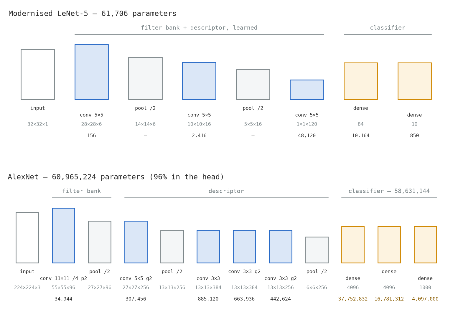
Figure 2.21 compares a modernised LeNet-5-style network with AlexNet, with every shape and parameter count computed from the formulas of this chapter.

A modernised LeNet-5-style network [4] reads \(32 \times 32\) digits. A \(5 \times 5\) convolution produces 6 maps of \(28 \times 28\) (156 parameters), followed by pooling to \(14 \times 14\). A second \(5 \times 5\) convolution produces 16 maps of \(10 \times 10\) (2,416 parameters), followed by pooling to \(5 \times 5\). A final \(5 \times 5\) convolution produces 120 maps of \(1 \times 1\) (48,120 parameters), followed by dense layers of 84 and 10 units (10,164 and 850 parameters). The total is 61,706.¹

AlexNet [1] has five convolutional layers with 96, 256, 384, 384, and 256 filters; three max pools; and dense layers of 4096, 4096, and 1000 units. The version diagrammed here takes a \(224 \times 224\) input and uses padding 2 in its first \(11 \times 11\), stride-4 convolution, producing a \(55 \times 55\) map. Without that padding, a \(227 \times 227\) input would be required to produce the same shape. Three of its convolutions are grouped with \(g = 2\), as the original two-GPU network had them, so the convolutional stack holds 2.3 million parameters rather than the 3.7 million a fully dense stack would need. The dense layers hold 58.6 million, so 96% of the 61.0 million parameters are in the head.

Figure 2.21: The template at two scales. Top: in a modernised LeNet-5, three convolutions and two pools take a \(32 \times 32\) digit to 120 channels at \(1 \times 1\), and a small dense head classifies. Bottom: in AlexNet, five convolutions and three pools take a \(224 \times 224\) photograph to 256 channels at \(6 \times 6\), and a dense head of 4096-4096-1000 units holds 96% of the parameters. Under each layer are its output shape and parameter count, from the formulas of this chapter, with the three layers marked g2 counted at \(g = 2\). The stage labels above are Chapter 1’s pipeline.

2.5.3 The head

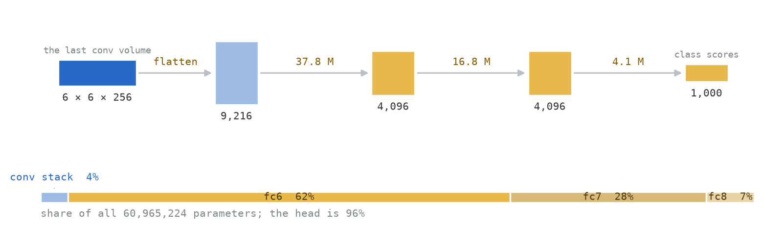
The convolutional stack ends with a volume; the task needs one number per class. The head is whatever converts one into the other, and the classical choice is to flatten the volume into a vector and follow it with dense layers. That choice is expensive. AlexNet’s final \(6 \times 6 \times 256\) volume flattens to 9,216 numbers, and connecting those to 4,096 dense units costs 37.8 million parameters in a single layer. Two more dense layers follow, and the three together hold 58.6 million of the network’s 61 million: the head carries 96% of the parameters, and the convolutional stack that does the seeing carries 4%. A dense layer’s count depends on the spatial size of its input, so the height-and-width independence that made the convolutional layers cheap does not apply here. Figure 2.22 draws the head and where its weights sit.

Figure 2.22: AlexNet’s dense head, drawn to scale by parameter count. The \(6 \times 6 \times 256\) volume flattens to a vector of 9,216, and three dense layers take it to 1,000 class scores. The first of them holds 37.8 million weights on its own, more than the whole convolutional stack, because every one of the 9,216 inputs connects to every one of the 4,096 units. The bars beneath give each layer’s share; the five convolutional layers together are the thin one on the left.

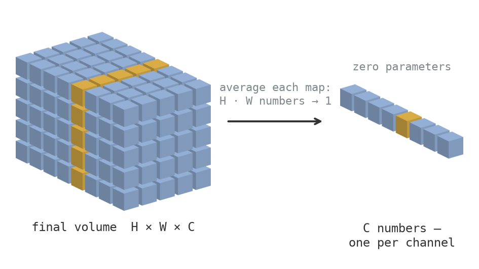
Global average pooling [10] replaces each channel of the final volume with its mean. An \(H \times W \times 256\) volume therefore becomes 256 numbers, with no learned parameters, before a dense layer maps them to the classes. Averaging discards the spatial arrangement and retains the mean response of each channel. If the preceding feature maps are translation equivariant, this converts translation equivariance into invariance. In a finite CNN, padding, strides, aliasing, and boundary effects make that invariance approximate. Because global average pooling accepts any spatial map size, a fully convolutional body can accept variable input resolutions above the minimum imposed by its kernels and downsampling layers. Figure 2.23 shows the operation.

Figure 2.23: Global average pooling. Each channel of the final volume, one of which is drawn in gold, collapses to its mean and fills one slot in a vector of \(C\) entries; position is gone. For AlexNet’s \(6 \times 6 \times 256\) volume that is 256 maps becoming 256 numbers, with zero parameters.

A dense layer applied to a \(6 \times 6 \times 256\) volume is a \(6 \times 6\) convolution with 4096 filters, and the parameter formula gives the same count either way. Read like that, the whole classifier is convolutions, and nothing stops it sliding: feed a larger image and the “classifier” produces its answer at every position, a map of dog-here. Detection and segmentation in Part II are built on that.

Interactive: count a network’s parameters

The two formulas of this chapter, applied to real networks. Open AlexNet and predict which row holds most of its 61 million parameters, then check against the gold row, which marks the most expensive. Then check the modernised LeNet-5: does the same imbalance hold at a thousandth of the size? Build your own stack and see what one dense layer does to the total.

2.5.4 Feature hierarchies

The first layer can be printed because its kernels have three channels, and three channels render as colour. That is the only reason Figure 2.2 could exist. A third-layer kernel is \(3 \times 3 \times 256\); there is nothing to print. Seeing what deep layers learned takes indirection: find the image patches that most excite a unit, or trace a response back to the pixels that produced it [11].

Many CNN classifiers develop a loose hierarchy of features [11]. First-layer filters often respond to edges and colour contrasts. Intermediate layers combine these responses into textures and parts, while later layers tend to be more task-specific and operate over wider receptive fields. The pattern depends on the architecture, dataset, and training objective, and not every channel has a simple semantic interpretation. Stacking the same type of learned layer allows the network to build these combinations without designing a new descriptor at each level, although additional layers still cost parameters and computation.

Figure 2.24 shows the hierarchy in the trained lab network, on the book’s scene.

Figure 2.24: The trained Lab 2 network looking at the scene, one layer per tab: each tile is one channel’s response map. Early maps fire on edges and colour boundaries anyone could have designed; deeper maps respond to fur, foliage, and configurations with no Chapter 1 counterpart. Click a map to lay it over the photograph and see what excites it.

2.6 Training

One question remains: where do the numbers come from? A trained AlexNet holds 61 million parameters, none of them set by hand. Three pieces fit them: a loss to say how wrong the network is, a gradient to say which way each parameter should move, and an optimiser to take the steps.

2.6.1 The loss

The network’s final layer produces one raw score per class, written \(z_c\) and called a logit. The softmax turns those scores into probabilities by exponentiating each, giving \(e^{z_c}\), and normalising by their sum:

\[ p_c = \frac{e^{z_c}}{\sum_j e^{z_j}}, \]

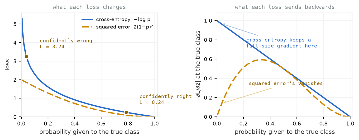
positive and summing to one. Training data supplies the true class, and the cross-entropy loss scores the network by the probability it gave that class: \(L = -\log p_{\text{true}}\). Confidently right costs nearly nothing; confidently wrong is punished without bound. A three-class example: logits \((2.0, -1.0, 0.5)\) give probabilities \((0.786, 0.039, 0.175)\). If the first class is true, \(L = -\log 0.786 = 0.24\); if the second, \(L = -\log 0.039 = 3.24\). One number says not just wrong but how confidently wrong.

Why not something simpler, like squared error against a one-hot target? Because its gradient, worked through the softmax, shrinks precisely when the network is most confidently wrong: the saturated cases that most need correcting are the ones squared error corrects most weakly. Cross-entropy’s gradient through the softmax is plain \(p - y\), large whenever the error is large. The loss is chosen for the gradient it sends backwards. Figure 2.25 draws the whole curve, with the two worked values on it.

Figure 2.25: Two losses on the same axis, for a two-class softmax where the probability given to the true class fixes everything. Left, what each loss charges: cross-entropy rises without bound as that probability goes to zero, while squared error against a one-hot target is capped at 2, so a confidently wrong answer is barely charged more than an uncertain one. The two marked points are the worked example, 0.24 and 3.24. Right, what each sends backwards: the size of the gradient arriving at the true class’s logit. Cross-entropy’s is \(1 - p\), largest exactly where the network is most confidently wrong; squared error’s is \(4p(1-p)^2\), which goes to zero there. At \(p = 0.02\) they are 0.98 and 0.077, a factor of thirteen. That gap, not the shape of the loss curve, is the reason for the choice.

2.6.2 Gradient descent, in batches

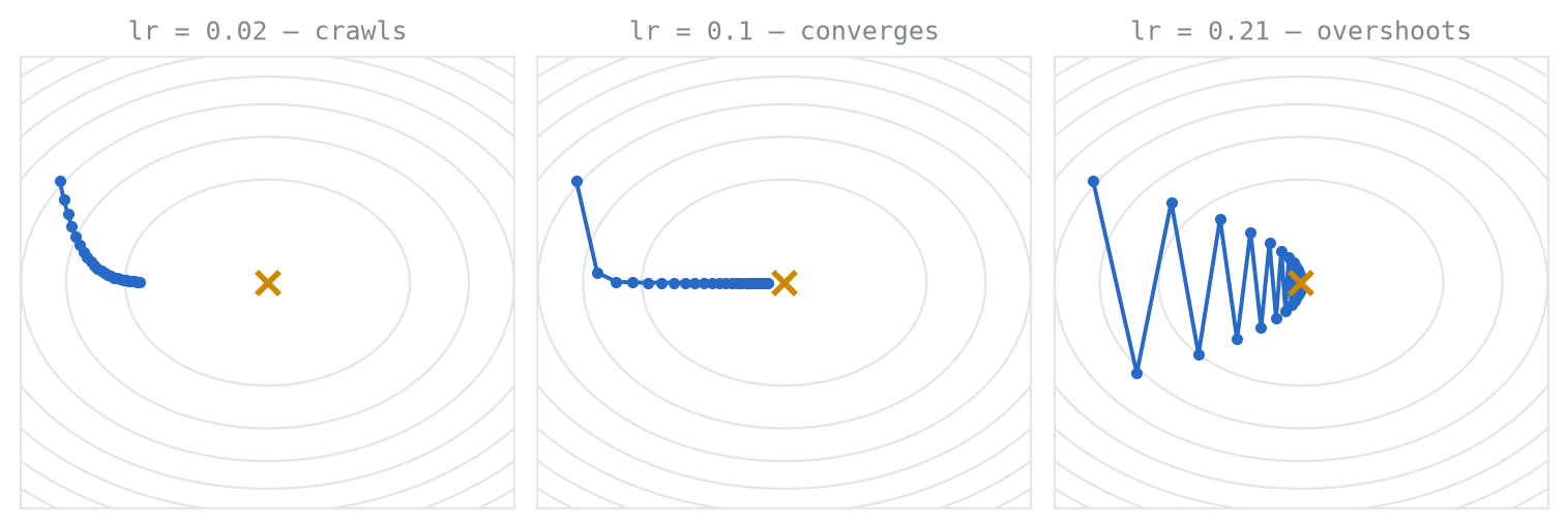
The loss is a single number depending on millions of parameters. The method is gradient descent: compute the gradient of the loss with respect to every parameter, and step each one a little downhill, \(\theta \leftarrow \theta - \eta \, \nabla_\theta L\). Computing the true gradient would mean the whole training set per step, so in practice each step uses a minibatch of, say, 128 images as a noisy estimate; one pass over the training set is an epoch. The noise is tolerable, and the saving in computation per step is what makes training feasible. This is stochastic gradient descent (SGD).

The step size \(\eta\) is the learning rate. If it is too small, optimisation proceeds slowly; if it is too large, updates can overshoot low-loss regions and the loss may oscillate or diverge. Momentum maintains an exponentially weighted sum of recent gradients and uses it to smooth the updates. Adam maintains running estimates of the gradients and their squares, using them to adapt the update for each parameter [12]. The lab uses Adam, but no optimiser removes the need to choose a suitable learning rate. Their relative performance depends on the model, data, and training setup. Many training runs reduce the learning rate over time, using a step schedule or cosine decay. Figure 2.26 shows the effects of three fixed learning rates.

Figure 2.26: Gradient descent on a two-parameter bowl at three step sizes, 24 steps each from the same start. Too small crawls and does not arrive. Right converges. Too large overshoots the narrow direction on every step and oscillates across the valley, which is the two-parameter version of a loss that jumps about.

2.6.3 Backpropagation

What remains is the gradient itself: the loss’s derivative with respect to every one of 61 million parameters, cheaply. The network is a chain of simple stages, so the chain rule applies stage by stage. Starting from the loss, each layer takes the gradient arriving at its output and produces two things: the gradient for its own weights, and the gradient at its input, which it hands to the layer below. One forward pass computes the network output, and one backward sweep computes every gradient. This is backpropagation. It is the same order of cost as the forward pass, but usually requires more arithmetic; for dense and convolutional layers, the backward computation is commonly about twice the forward computation. Figure 2.27 shows the two passes.

Figure 2.27: The two passes through one network. Forward (blue): each layer hands its output to the next, ending in the loss. Backward (gold): each layer takes the gradient arriving from above, keeps the part belonging to its own weights, and hands the rest down.

ImportantThe chain rule, stated once

For a two-stage network \(L = f(g(\theta))\), the chain rule gives \(\partial L / \partial \theta = f'(g(\theta)) \cdot g'(\theta)\). A deep network is the same statement iterated: writing \(a_\ell\) for layer \(\ell\)’s output, \[ \frac{\partial L}{\partial a_{\ell-1}} = \frac{\partial a_{\ell}}{\partial a_{\ell-1}}^{\!\top} \frac{\partial L}{\partial a_{\ell}}, \qquad \frac{\partial L}{\partial \theta_{\ell}} = \frac{\partial a_{\ell}}{\partial \theta_{\ell}}^{\!\top} \frac{\partial L}{\partial a_{\ell}}. \] Each layer needs only its local Jacobians; the product of the chain is assembled by the backward sweep. Every factor in that product is a matrix, and Chapter 3 opens with what happens to long products of matrices.

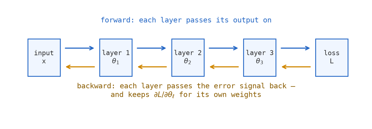
During backpropagation through a convolution, the layer computes two derivatives. The gradient with respect to its input, \(\partial L / \partial x\), applies the transpose of the forward operator and is passed to the preceding layer. The gradient with respect to its kernel weights, \(\partial L / \partial W\), correlates the stored input with the gradient arriving at the layer’s output. The optimiser uses this second gradient to update the weights.

PyTorch’s autograd records the forward operations and computes their gradients during the backward pass. Before a full training run, overfit a single batch: disable data augmentation and regularisation, then train repeatedly on one fixed batch. This checks that the model can memorise the examples and that the data, model, loss, and optimiser are connected correctly. The network should reach 100% accuracy and a very small loss on the batch. If it cannot, fix that problem before training on the full dataset.

2.6.4 Initialisation

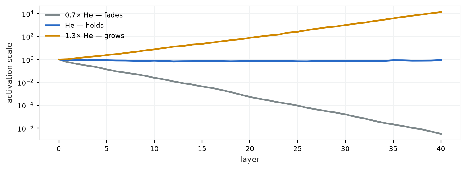
Biases can be initialised to zero, but the filters in a layer must not all start with identical weights. Identical filters receive identical gradients and remain identical during training, so their weights are initialised randomly. The scale also matters. If it is too small, activations and gradients shrink through the network; if it is too large, they can grow until training becomes numerically unstable. ReLU does not saturate for positive inputs, but it does not prevent this growth. He initialisation [13] uses zero-mean weights with variance

\[ \frac{2}{k^2 C_{\text{in}}} \]

for a convolutional ReLU layer. This keeps the activation scale approximately stable at the start of training. Figure 2.28 shows the effect through a 40-layer stack.

Figure 2.28: What the initial weight scale does to the signal, computed for a 40-layer ReLU stack of width 256. At He scale the activation magnitude holds; at 0.7× it decays to about \(3 \times 10^{-7}\) and at 1.3× it grows past \(10^{4}\). Either way, by the bottom of a deep stack there is nothing sensible left to train.

NoteHow precise must the scale be?

He initialisation is a safe default, but exact critical initialisation is not always necessary. Pretorius and colleagues trained more than 12,000 shallow-to-moderate ReLU networks and found no statistically significant performance difference over a broad range of non-critical initialisations. Only very small or very large scales performed consistently worse [14]. The figure above describes signal propagation at initialisation; it does not imply that small deviations from the He scale prevent a moderate-depth network from training.

2.6.5 Regularisation

A model is overfitting when its training performance continues to improve while its validation performance stalls or worsens. Common countermeasures include weight decay, dropout, early stopping, and data augmentation. AlexNet used weight decay, dropout, and data augmentation [1].

Weight decay penalises large weights, commonly by adding a term proportional to \(\lVert \theta \rVert^2\) to the loss. With ordinary SGD, this pulls each weight towards zero on every update.

Dropout [15] sets activations to zero independently with probability \(p\) during training. In PyTorch’s inverted-dropout convention, the retained activations are divided by \(1-p\) during training, so evaluation requires no rescaling.

Early stopping retains the parameters from the epoch with the best validation performance. It limits how long the model can adapt to details specific to the training set.

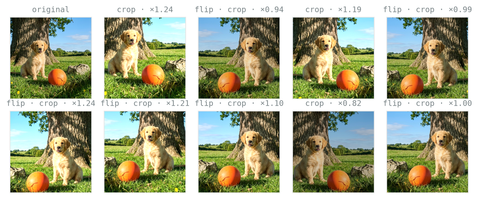
Data augmentation trains on transformed examples that retain the same label, such as flips, crops, and small colour changes. It encourages the network to produce similar outputs for those transformations, but does not create exact invariance. A standard CNN has no built-in equivariance to rotation, scale, or changes in illumination, while its translation equivariance is limited by padding, strides, and boundaries, as discussed above. The lab uses random flips and crops; augmentation pipelines receive fuller treatment in the next chapter. Figure 2.29 shows examples.

Figure 2.29: One crop of the scene, and nine augmented copies the network might see instead: flips, shifted crops, and brightness scaled by the factor in each title. Every copy keeps the label dog.

2.6.6 Reading the curves

Training and validation curves provide symptoms, not unique diagnoses. Figure 2.30 shows four controlled runs of the same network. In the healthy run, both accuracies rise with a modest gap. In the overfitting run, training accuracy reaches 100% while validation accuracy stalls. The low-learning-rate run improves slowly, while the high-learning-rate run remains near chance. Other faults can produce similar curves, so diagnose them by checking the configuration and changing one factor at a time.

Figure 2.30: Four training runs of the Lab 2 network on CIFAR-10, identical but for the labelled change (the overfitting run gets 500 epochs, because its small training set needs the extra passes before the gap opens fully). Healthy (lr = 0.01, momentum, augmentation): both accuracies climb, small gap. Overfit (2,000-image training set, no augmentation): training accuracy reaches 100% while validation stops at 56%. Too low (lr = 10⁻⁴): the same rise at a fraction of the pace. Too high (lr = 1.0): every step overshoots, and accuracy never leaves chance. Hover any epoch to read both curves and the gap between them. Switch to loss and the overfitting run shows the other half of its signature, a validation loss that climbs while the training loss falls towards zero.

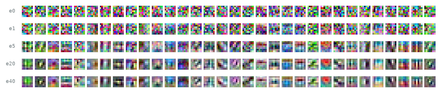
The filters change over those same epochs. Figure 2.31 prints the first layer at initialisation and after 1, 5, 20, and 40 epochs: random static organising itself, epoch by epoch, into oriented edges and colour contrasts.

Figure 2.31: First-layer filters across training: at initialisation and after 1, 5, 20, and 40 epochs on CIFAR-10. Structure emerges from random weights under nothing but the classification loss, giving smaller, blurrier relatives of the AlexNet filters in Figure 2.2. The network is the lab’s, with its first layer widened from \(3 \times 3\) to \(7 \times 7\) so the filters are legible at this size.

Interactive: train one yourself

A small CNN, a small digit set, training live. Set the learning rate an order of magnitude too high, predict which curve shape from Figure 2.30 you will get, and run it; then find the largest rate that still trains cleanly. The first-layer filters update as it runs; note the epoch at which structure first appears.

2.7 The learned filter bank

Figure 2.2 can now be read as a learned filter bank. Its \(11 \times 11 \times 3\) kernels can be displayed directly because the input has three colour channels. Their Gabor-like patterns emerged from random initial weights under the classification loss. A CNN does not explicitly learn a Gaussian \(\sigma\), a Sobel kernel, or the members of an MR8 bank. It learns unconstrained kernels and intermediate representations jointly with the classifier. Some first-layer kernels resemble classical filters because edges, colour contrasts, and oriented patterns are useful for the task.

The deeper layers are the part with no Chapter 1 counterpart at all: nothing in the design says what layer five should compute. A loss at the top and a gradient path to the bottom were enough.

One fact about these filters is left unexplained. They were fitted to a single dataset and a single task: 1.2 million photographs, 1,000 nouns. Yet the first layers keep rediscovering Gabor filters, which were designed with no dataset at all. How much of what this network learned is about ImageNet, and how much is about images? Chapter 3 takes that question up directly.

Exercises

1. Reading learned filters. Pick four filters from Figure 2.2: one oriented achromatic filter, one colour-opponent filter, and two of your choice. For each, say what image structure maximises its response, and name its nearest relative in the MR8 bank, or state that it has none, and why.
2. Parameter counting. A network for \(32 \times 32 \times 3\) inputs: conv \(3 \times 3\), 32 filters; conv \(3 \times 3\), 32 filters; max pool 2; conv \(3 \times 3\), 64 filters; conv \(1 \times 1\), 16 filters; global average pool; dense to 10 classes. Count the parameters of every layer, then count a single dense layer from the flattened input to 10 classes, and compare.
3. Receptive fields. For the stack conv \(5 \times 5\)/1, pool \(2 \times 2\)/2, conv \(3 \times 3\)/1, conv \(3 \times 3\)/1, pool \(2 \times 2\)/2, conv \(3 \times 3\)/1, compute the receptive field and jump after every layer. A pedestrian is 96 pixels tall. Assume the final feature map has 64 channels. Without adding further downsampling, extend the stack using \(3 \times 3\), stride-1 convolutions that map 64 channels to 64 channels and include a bias. How many layers are required for one top-layer unit to see all 96 pixels, and how many parameters do they add?
4. Choosing from the zoo. For each requirement, name the variant and show the arithmetic, ignoring biases throughout: (a) an output map at twice the input resolution; (b) a \(9 \times 9\) receptive field from nine weights; (c) the parameter count of a \(3 \times 3\), 256-to-256 layer cut by a factor of four, accepting the loss of channel mixing across groups of 64; (d) the same layer cut roughly ninefold, channel mixing preserved.
5. Shapes through a modernised LeNet-5. Reproduce the modernised LeNet-5 table of Figure 2.21 from the two formulas alone: every output shape and every parameter count, given only the layer specifications in the text.
6. One step, by hand. Logits \((1.0, 3.0)\), true class 1 (the first). Compute the softmax, the cross-entropy loss, and the gradient \(p - y\) at the logits. Then, for a 1-D convolution with kernel \([w_1, w_2]\) on input \([x_1, x_2, x_3]\), write the two outputs, and use the chain rule to express \(\partial L / \partial w_1\) in terms of the output gradients.
7. Diagnosis. Four runs are described: (a) training accuracy 99%, validation 62%; (b) both accuracies at 10% after twenty epochs, loss unchanged from its initial value; (c) both curves improving smoothly, training a steady 3% ahead; (d) loss alternating between 1.2 and 6.0 from epoch to epoch. Diagnose each and propose the single change you would try first.
8. The audit, rerun. Rerun the invariance audit for a CNN. First assess the exact architectural properties of: a stride-1 convolutional stack; the stack after pooling or strided convolution; and the network after global average pooling. Account for padding, boundaries, and aliasing. Then consider a network trained with flip-and-crop augmentation: which transformations should it become more robust to, and does the augmentation provide an exact guarantee? Consider translation, rotation, uniform scaling, and horizontal reflection.

Lab 2

Lab 2: a small CNN on CIFAR-10 from scratch; compare to an MLP; visualise the learned first-layer filters next to Chapter 1’s Gabor bank. W&B logging from the first run; seed everything; overfit a single batch before training for real.

Open in Colab

Further reading

• LeCun et al. [4] — LeNet-5, and a strikingly complete statement of the whole programme, fourteen years early.
• Krizhevsky, Sutskever, and Hinton [1] — AlexNet; short, readable, and the origin of half this chapter’s numbers.
• Zeiler and Fergus [11] — what the layers learn, and how anyone found out.
• Dumoulin and Visin [7] — the convolution-arithmetic reference the zoo widget animates.
• Zhang [5] — the aliasing callout, taken seriously and fixed.
• Goodfellow, Bengio, and Courville [16], chapter 9 — the formal treatment of everything here; free online.

References

[1]

A. Krizhevsky, I. Sutskever, and G. E. Hinton, “ImageNet classification with deep convolutional neural networks,” in Advances in neural information processing systems (NIPS), 2012, pp. 1097–1105.

[2]

O. Russakovsky et al., “ImageNet large scale visual recognition challenge,” International Journal of Computer Vision, vol. 115, no. 3, pp. 211–252, 2015, doi: 10.1007/s11263-015-0816-y.

[3]

K. Fukushima, “Neocognitron: A self-organizing neural network model for a mechanism of pattern recognition unaffected by shift in position,” Biological Cybernetics, vol. 36, no. 4, pp. 193–202, 1980, doi: 10.1007/BF00344251.

[4]

Y. LeCun, L. Bottou, Y. Bengio, and P. Haffner, “Gradient-based learning applied to document recognition,” Proceedings of the IEEE, vol. 86, no. 11, pp. 2278–2324, 1998, doi: 10.1109/5.726791.

[5]

R. Zhang, “Making convolutional networks shift-invariant again,” in International conference on machine learning (ICML), 2019, pp. 7324–7334.

[6]

W. Luo, Y. Li, R. Urtasun, and R. Zemel, “Understanding the effective receptive field in deep convolutional neural networks,” in Advances in neural information processing systems (NIPS), 2016, pp. 4898–4906.

[7]

V. Dumoulin and F. Visin, “A guide to convolution arithmetic for deep learning,” arXiv preprint arXiv:1603.07285, 2016, Available: https://arxiv.org/abs/1603.07285

[8]

A. Odena, V. Dumoulin, and C. Olah, “Deconvolution and checkerboard artifacts,” Distill, 2016, doi: 10.23915/distill.00003.

[9]

S. Xie, R. Girshick, P. Dollár, Z. Tu, and K. He, “Aggregated residual transformations for deep neural networks,” in IEEE conference on computer vision and pattern recognition (CVPR), 2017, pp. 1492–1500. doi: 10.1109/CVPR.2017.634.

[10]

M. Lin, Q. Chen, and S. Yan, “Network in network,” in International conference on learning representations (ICLR), 2014. Available: https://arxiv.org/abs/1312.4400

[11]

M. D. Zeiler and R. Fergus, “Visualizing and understanding convolutional networks,” in European conference on computer vision (ECCV), 2014, pp. 818–833. doi: 10.1007/978-3-319-10590-1_53.

[12]

D. P. Kingma and J. Ba, “Adam: A method for stochastic optimization,” in International conference on learning representations (ICLR), 2015. Available: https://arxiv.org/abs/1412.6980

[13]

K. He, X. Zhang, S. Ren, and J. Sun, “Delving deep into rectifiers: Surpassing human-level performance on ImageNet classification,” in IEEE international conference on computer vision (ICCV), 2015, pp. 1026–1034. doi: 10.1109/ICCV.2015.123.

[14]

A. Pretorius et al., “If dropout limits trainable depth, does critical initialisation still matter? A large-scale statistical analysis on ReLU networks,” Pattern Recognition Letters, vol. 138, pp. 95–105, 2020, doi: 10.1016/j.patrec.2020.06.025.

[15]

N. Srivastava, G. Hinton, A. Krizhevsky, I. Sutskever, and R. Salakhutdinov, “Dropout: A simple way to prevent neural networks from overfitting,” Journal of Machine Learning Research, vol. 15, pp. 1929–1958, 2014, Available: https://jmlr.org/papers/v15/srivastava14a.html

[16]

I. Goodfellow, Y. Bengio, and A. Courville, Deep learning. MIT Press, 2016. Available: https://www.deeplearningbook.org/

---

1. The published LeNet-5 has 60,000 trainable parameters. Its C3 layer is sparsely connected, its subsampling layers have trainable scales and biases, and its output uses fixed radial-basis-function prototypes. The version counted here uses full channel connectivity, parameter-free pooling, and a learned affine output layer.