5 Basics
5.1 Coordinate Systems
A coordinate system is a framework used to uniquely identify and describe the position of points or other geometric elements in a given space. It provides a standardized method for defining and referencing locations in one, two, three, or higher dimensions. Here are the key aspects and types of coordinate systems:
Key Aspects of Coordinate Systems
Reference Origin: A fixed point in the coordinate system, often denoted as the origin (e.g., (0, 0) in 2D, (0, 0, 0) in 3D), from which all measurements are made.
Axes: Lines that intersect at the origin and extend in various directions. The axes are used as reference lines to measure distances and angles. In a Cartesian coordinate system, these are typically the x-axis, y-axis, and z-axis.
Coordinates: Ordered sets of numbers that define the position of a point relative to the axes and origin. For example, in 2D Cartesian coordinates, a point is represented as (x, y).
Dimensions: The number of independent directions in which movement is possible within the space. Commonly, 1D (line), 2D (plane), and 3D (space) coordinate systems are used.
5.1.1 Pixel Coordinates
A digital image is made up of rows and columns of pixels.
A pixel in such an image can be specified by saying which column and which row contains it. In terms of coordinates, a pixel can be identified by a pair of integers giving the column number and the row number.
For example, the pixel with coordinates (3,5) would lie in column number 3 and row number 5.
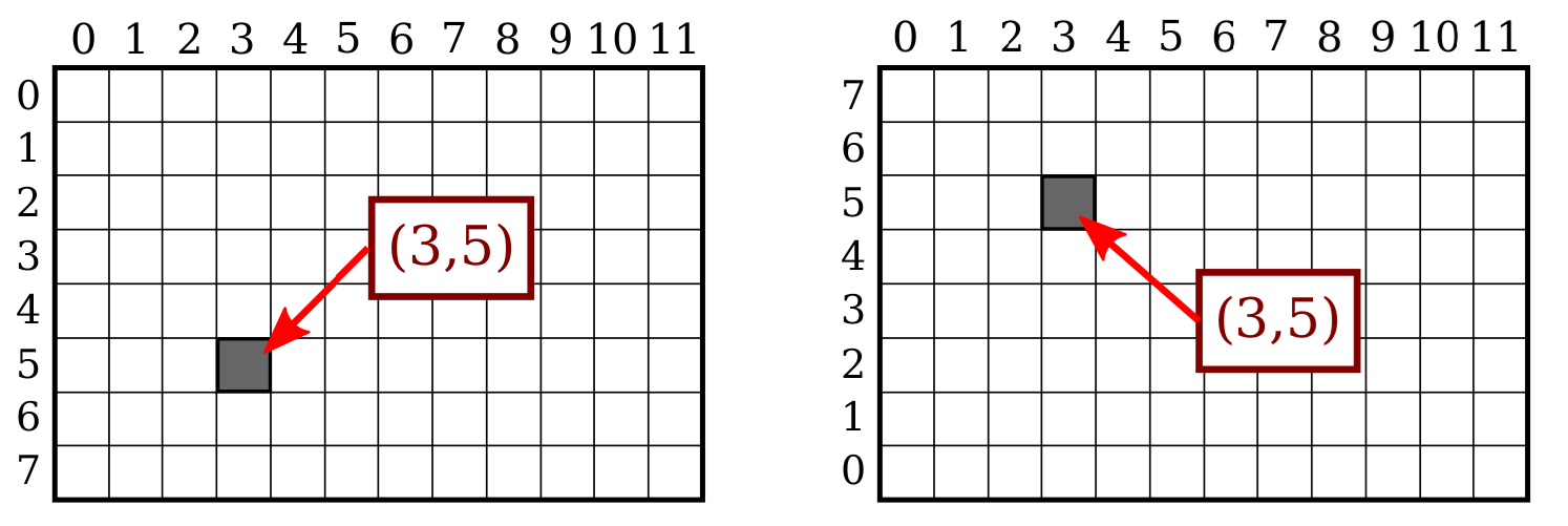
Conventionally, columns are numbered from left to right, starting with zero. Most graphics systems, including the ones we will study in this course, number rows from top to bottom, starting from zero. Some, including OpenGL, number the rows from bottom to top instead.
5.1.1.1 Drawing Lines
Suppose, for example, that we want to draw a line segment. A mathematical line has no thickness and would be invisible. So we really want to draw a thick line segment, with some specified width. Let’s say that the line should be one pixel wide.
The problem is that, unless the line is horizontal or vertical, we can’t actually draw the line by coloring pixels.

A diagonal geometric line will cover some pixels only partially. It is not possible to make part of a pixel black and part of it white. When you try to draw a line with black and white pixels only, the result is a jagged staircase effect.
 This effect is an example of something called “aliasing.” Aliasing can also be seen in the outlines of characters drawn on the screen and in diagonal or curved boundaries between any two regions of different colour.
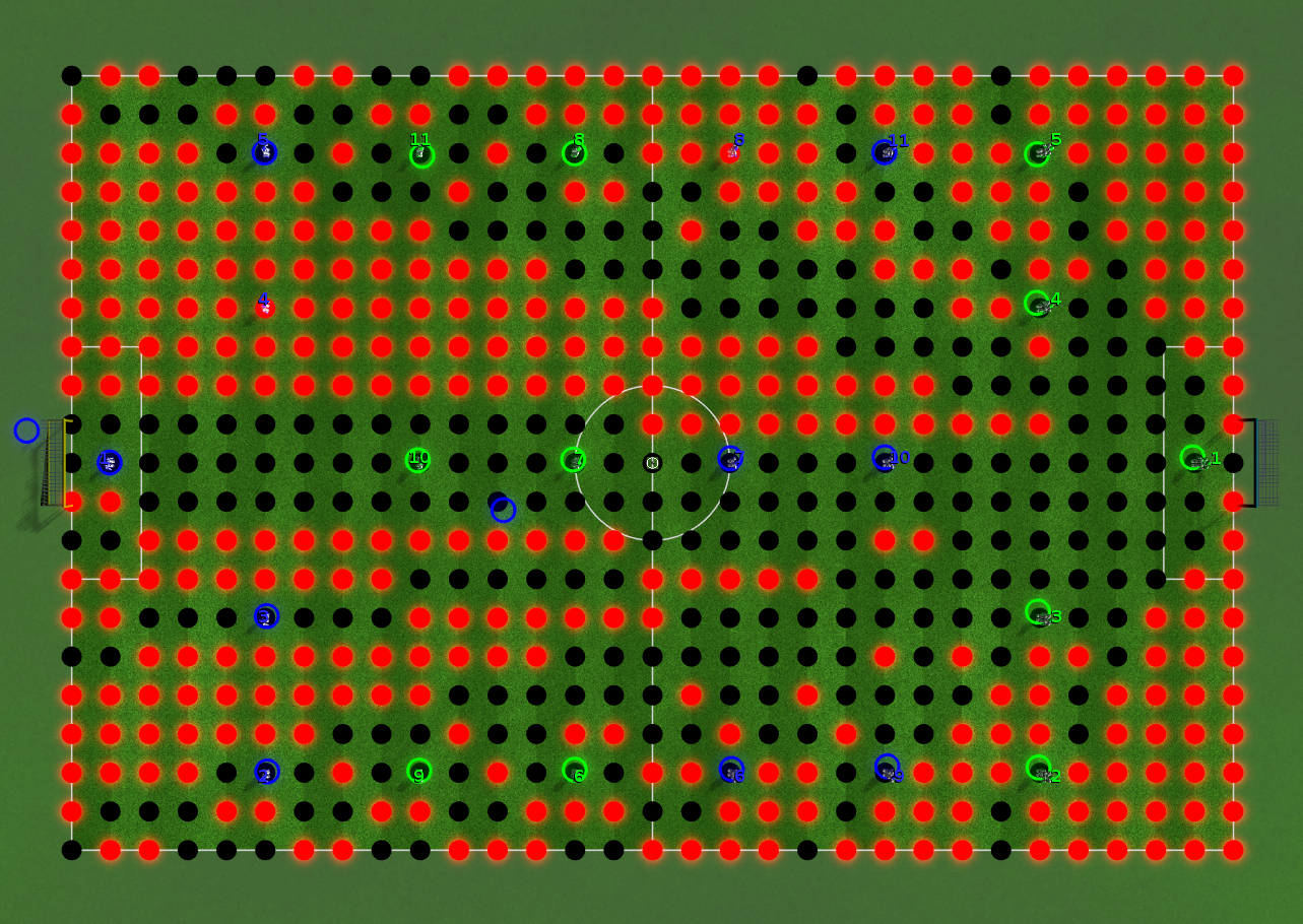
There are many different algorithms which are used for line drawing in computers one example is the Bresenham Line drawing algorithm which finds the discrete set of pixels between two points.
This algorithm is actually used in WITS’s Robocup team in order to identify regions which obstructed. In particular we use the goal mouth as the start location and the opponents positions as then end position such that each position between those locations is considered Obstructed, this can be seen in the following image where the red dots indicated unobstructed regions and the black dots are obstructed regions. Additionally in this figure the Opponents are located by the green circles and our players are located by the blue circles.
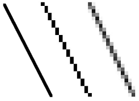
Antialiasing is a term for techniques that are designed to mitigate the effects of aliasing. The idea is that when a pixel is only partially covered by a shape, the color of the pixel should be a mixture of the color of the shape and the color of the background. When drawing a black line on a white background, the color of a partially covered pixel would be gray, with the shade of gray depending on the fraction of the pixel that is covered by the line. (In practice, calculating this area exactly for each pixel would be too difficult, so some approximate method is used.) Here, for example, is a geometric line, shown on the left, along with two approximations of that line made by coloring pixels. The lines are greatly magnified so that you can see the individual pixels. The line on the right is drawn using antialiasing, while the one in the middle is not
There are many different algorithms which are used for anti-aliasing applied at different points in the rendering pipeline
5.1.2 Real Value Coordinates
The coordinates for a pixel will, in general, be real numbers rather than integers. In fact, it’s better to forget about pixels and just think about points in the image. A point will have a pair of coordinates given by real numbers. To specify the coordinate system on a rectangle, you just have to specify the horizontal coordinates for the left and right edges of the rectangle and the vertical coordinates for the top and bottom. Let’s call these values left, right, top, and bottom. Often, they are thought of as xmin, xmax, ymin, and ymax, but there is no reason to assume that, for example, top is less than bottom.
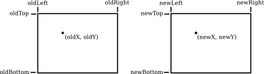
In order to move from one coordinate space to another we apply a transform on the original space.
The formula to transform the x-coordinate is given by:
\[ \text{newX} = \text{newLeft} + \frac{\text{oldX} - \text{oldLeft}}{\text{oldRight} - \text{oldLeft}} \times (\text{newRight} - \text{newLeft}) \]
The formula to transform the y-coordinate is given by:
\[ \text{newY} = \text{newTop} + \frac{\text{oldY} - \text{oldTop}}{\text{oldBottom} - \text{oldTop}} \times (\text{newBottom} - \text{newTop}) \]
5.1.2.1 Explanation
-
Old Rectangle: Defined by boundaries
oldLeft,oldRight,oldTop, andoldBottom. -
New Rectangle: Defined by boundaries
newLeft,newRight,newTop, andnewBottom. - Point Mapping: The point \((\text{oldX}, \text{oldY})\) in the old rectangle is mapped to \((\text{newX}, \text{newY})\) in the new rectangle using the transformation formulas.
- These formulas linearly interpolate the coordinates of the point, preserving the relative position of the point within the rectangle.
By using these formulas, you can transform any point from one rectangle to another, maintaining its relative position.
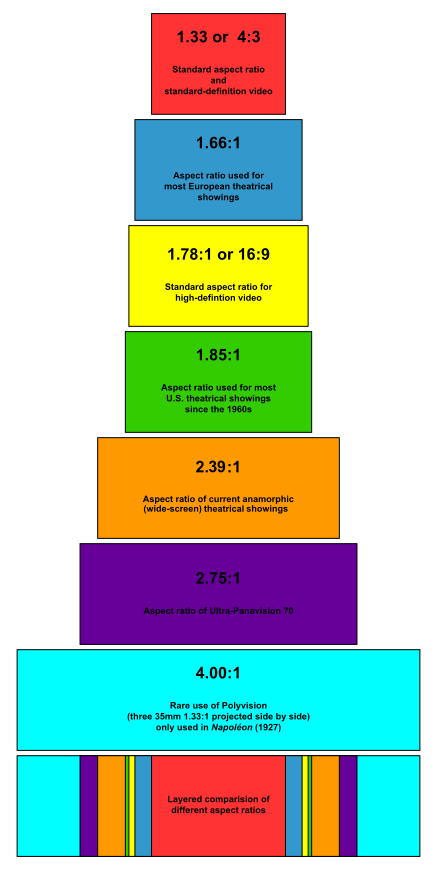
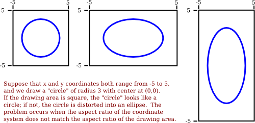
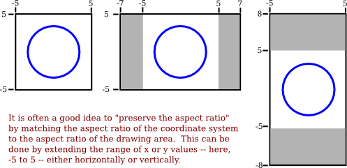
5.1.2.2 Aspect Ratio
The aspect ratio of an image is the ratio of its width to its height. It defines the shape of the image and is crucial in maintaining the visual proportions of graphics across different devices and screens.
Common aspect ratios include 4:3, 16:9, and 21:9. Properly managing aspect ratios ensures that images and videos display correctly without distortion.
5.2 Colours
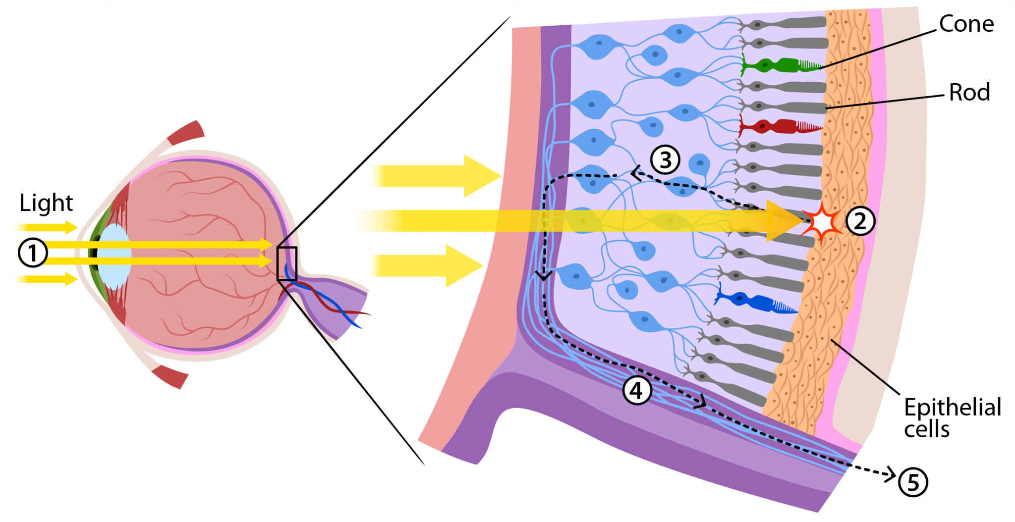
Light is made up of waves with a variety of wavelengths. A pure color is one for which all the light has the same wavelength, but in general, a color can contain many wavelengths.
You might have heard that combinations of the three basic, or “primary,” colors are sufficient to represent all colors, because the human eye has three kinds of color sensors that detect red, green, and blue light. However, that is only an approximation. The eye does contain three kinds of color sensors. The sensors are called “cone cells.” However, cone cells do not respond exclusively to red, green, and blue light.
The colours on a computer screen are produced as combinations of red, green, and blue light. Different colors are produced by varying the intensity of each type of light.
5.2.1 Alpha
Often, a fourth component is added to color models. The fourth component is called alpha, and color models that use it are referred to by names such as RGBA and HSLA. Alpha is not a color as such. It is usually used to represent transparency.
A color with maximal alpha value is fully opaque; that is, it is not at all transparent. A color with alpha equal to zero is completely transparent and therefore invisible. Intermediate values give translucent, or partly transparent, colors. Transparency determines what happens when you draw with one color (the foreground color) on top of another color (the background color). If the foreground color is fully opaque, it simply replaces the background color. If the foreground color is partly transparent, then it is blended with the background color. Assuming that the alpha component ranges from 0 to 1, the color that you get can be computed as
new_color = (alpha)*(foreground_color) + (1 - alpha)*(background_color)This computation is done separately for the red, blue, and green color components. This is called alpha blending. The effect is like viewing the background through colored glass; the color of the glass adds a tint to the background color
5.3 Shapes
Shapes are fundamental elements in computer graphics, used to create and define visual content. Basic shapes include circles, squares, triangles, and more complex polygons. All these basic shapes are made up of connecting line segments
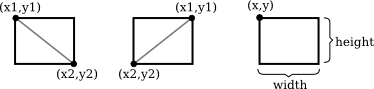
The basic rectangular shape has sides that are vertical and horizontal. (A tilted rectangle generally has to be made by applying a rotation.) Such a rectangle can be specified with two points, (x1,y1) and (x2,y2), that give the endpoints of one of the diagonals of the rectangle. Alternatively, the width and the height can be given, along with a single base point, (x,y). In that case, the width and height have to be positive, or the rectangle is empty. The base point (x,y) will be the upper left corner of the rectangle if y increases from top to bottom, and it will be the lower left corner of the rectangle if y increases from bottom to top.
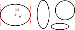
An oval with this property can be specified by giving the rectangle that just contains it. Or it can be specified by giving its center point and the lengths of its vertical radius and its horizontal radius. In this illustration, the oval on the left is shown with its containing rectangle and with its center point and radii:
If ovals are not available as basic shapes, they can be approximated by drawing a large number of line segments. The number of lines that is needed for a good approximation depends on the size of the oval. It’s useful to know how to do this. Suppose that an oval has center point (x,y), horizontal radius r1, and vertical radius r2. Mathematically, the points on the oval are given by
where angle takes on values from 0 to 360 if angles are measured in degrees or from 0 to 2π if they are measured in radians. Here sin and cos are the standard sine and cosine functions. To get an approximation for an oval, we can use this formula to generate some number of points and then connect those points with line segments. In pseudocode, assuming that angles are measured in radians and that pi represents the mathematical constant π,
Draw Oval with center (x,y), horizontal radius r1, and vertical radius r2:
      for i = 0 to numberOfLines:
           angle1 = i * (2*pi/numberOfLines)
           angle2 = (i+1) * (2*pi/numberOfLines)
           a1 = x + r1*cos(angle1)
           b1 = y + r2*sin(angle1)
           a2 = x + r1*cos(angle2)
           b2 = y + r2*sin(angle2)
           Draw Line from (a1,b1) to (a2,b2)
5.4 Line Properties
Lines can have other attributes, or properties, that affect their appearance. One question is, what should happen at the end of a wide line? Appearance might be improved by adding a rounded “cap” on the ends of the line. A square cap—that is, extending the line by half of the line width—might also make sense. Another question is, when two lines meet as part of a larger shape, how should the lines be joined? And many graphics systems support lines that are patterns of dashes and dots.

5.5 Stroke vs Fill
In computer graphics, ‘stroke’ refers to the outline of a shape, while ‘fill’ refers to the interior. The stroke can have properties such as color, width, and style (solid, dashed), whereas the fill can be a solid color, gradient, or pattern.
Filling a shape means coloring all the points that are contained inside that shape. When a shape intersects itself, like the two shapes in the illustration below, it’s not entirely clear what should count as the interior of the shape. In fact, there are at least two different rules for filling such a shape. Both are based on something called the winding number. The winding number of a shape about a point is, roughly, how many times the shape winds around the point in the positive direction, which I take here to be counterclockwise. Winding number can be negative when the winding is in the opposite direction.
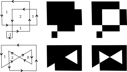
The shapes above are shown filled using the two fill rules. For the shapes in the center, the fill rule is to color any region that has a non-zero winding number. For the shapes shown on the right, the rule is to color any region whose winding number is odd; regions with even winding number are not filled.
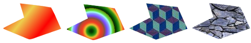
Shapes can be filled with color, gradients, or textures to add depth and interest to graphics.
5.6 Polygons, Curves and Paths
Polygons are multi-sided shapes with straight edges, while curves are smooth, flowing lines that can be defined by mathematical functions. Paths are combinations of lines and curves that define complex shapes. These elements are crucial in vector graphics, where they are used to create scalable images that retain quality at any size.

A path is created by giving a series of commands that tell, essentially, how a pen would be moved to draw the path. While a path is being created, there is a point that represents the pen’s current location. There will be a command for moving the pen without drawing, and commands for drawing various kinds of segments.
createPath() — start a new, empty path
moveTo(x,y) — move the pen to the point (x,y), without adding a segment to the path; that is, without drawing anything
lineTo(x,y) — add a line segment to the path that starts at the current pen location and ends at the point (x,y), and move the pen to (x,y)
closePath() — add a line segment from the current pen location back to the starting point, unless the pen is already there, producing a closed path.
A path represents an abstract geometric object. Creating one does not make it visible on the screen. Once we have a path, to make it visible we need additional commands for stroking and filling the path.
5.6.1 Bezier curve
A path can contain other kinds of segments besides lines. For example, it might be possible to include an arc of a circle as a segment. Another type of curve is a Bezier curve. A smooth curve between two points defined by parametric polynomial equations.
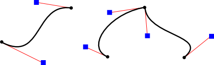
Bezier curves can be used to create very general curved shapes. They are fairly intuitive, so that they are often used in programs that allow users to design curves interactively in order to make complex shapes as seen in the scene below.
A cubic Bezier curve segment is defined by its two endpoints P1 and P2 and by two control points C1 and C2. The tangent to the curve (its direction and speed) at P1 is given by the line from P1 to C1. The tangent vector to the curve at P2 is given by the line from C2 to P2. A quadratic Bezier curve is defined by its two endpoints and a single control point C. The tangent at each endpoint is the line between that endpoint and C.
The Bézier Game. A game to help you master the pen tool. This game requires keyboard and mouse.
5.7 Modelling and Viewing
Modelling and Viewing are two fundamental concepts in computer graphics, each serving a distinct purpose in the process of rendering a 3D scene onto a 2D display.
5.7.1 Modelling
- Definition: Modelling refers to the process of creating and defining the shapes, structures, and properties of objects within a 3D space. This involves specifying the object’s geometry using coordinates in what is known as the object coordinate system.
- Object Coordinates: These are the coordinates used to define the shape and structure of an object in its own local space. For example, a cube may be defined with vertices at (±1, ±1, ±1) in object coordinates.
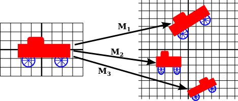
- Modelling Transformation: Once an object is defined, it needs to be positioned, oriented, and scaled appropriately within a larger scene. This is achieved through a series of transformations (translation, rotation, scaling) that convert object coordinates into world coordinates. This process is known as the modelling transformation.
- Purpose: The goal of modelling is to accurately represent the objects in a scene with their inherent properties, independent of their position or orientation in the final scene.
5.7.2 Viewing
- Definition: Viewing refers to the process of defining how the scene is observed, or viewed, by a camera. This involves specifying the viewpoint, direction, and perspective from which the scene is rendered.
- Viewport: The viewport is the rectangular area on the display device where the final rendered image is shown. It acts like a window through which the scene is viewed.
-
Viewing Transformation: This includes transforming world coordinates into camera coordinates, and eventually into screen coordinates. The viewing transformation typically involves:
- Camera Transformation: Positioning and orienting the camera within the world coordinate system.
- Projection Transformation: Converting the 3D coordinates into 2D coordinates, applying perspective or orthographic projection.
- Viewport Transformation: Mapping the 2D coordinates to the appropriate location on the screen or window.
- Purpose: The viewing process determines how the scene is visualized, including what portion of the scene is visible, how it is framed, and how the 3D objects are projected onto a 2D plane.
5.8 Transformations
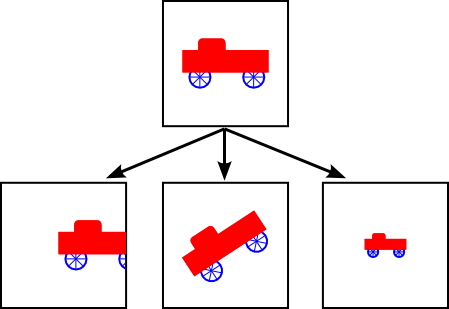
Transformations are operations that modify the position, size, and orientation of objects in a coordinate space. They are fundamental in computer graphics for manipulating objects and creating animations.
The transforms we will use in 2D graphics can be written in the form
where (x,y) represents the coordinates of some point before the transformation is applied, and (x1,y1) are the transformed coordinates. The transform is defined by the six constants a, b, c, d, e, and f. Note that this can be written as a function T, where
A transformation of this form is called an Affine Transform. This notation should be familiar as you have long studied Linear Transformations.
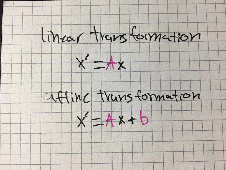
An affine transform has the property that, when it is applied to two parallel lines, the transformed lines will also be parallel. Also, if you follow one affine transform by another affine transform, the result is again an affine transform.
In the context of affine transformations, we often extend 2D coordinates to 3D homogeneous coordinates by adding a third component, set to 1. This allows us to represent 2D transformations, including translations, as matrix multiplications.
The typical coordinate (x,y) becomes (x,y,1) in homogeneous coordinates. The extension to three components allows us to incorporate translation into the matrix form, which wouldn’t be directly possible in a purely linear transformation matrix (limited to rotation, scaling, shearing). The bottom row [0,0,1] ensures that the third component of the homogeneous coordinate remains 1 after the transformation. This is essential for keeping the system consistent and ensuring the translation part of the matrix works correctly.
If the bottom row were different, say [0,0,0], the third component of all transformed points would turn to zero, effectively making the homogeneous coordinate invalid for practical purposes. Moreover, a zero or other value instead of one would prevent proper scaling and repositioning of the point after translation.
5.8.1 Translation
Translation moves an object from one position to another in a straight line. This is done by adding a translation vector to the coordinates of the object. If (x,y) is the original point and (x1,y1) is the transformed point, then the formula for a translation is
where e is the number of units by which the point is moved horizontally and f is the amount by which it is moved vertically. Thus for a translation, a = d = 1, and b = c = 0 in the general formula for an affine transform. A 2D graphics system will typically have a function such as
This can be represented by the following transformation matrix: \[ \begin{bmatrix} 1 & 0 & t_x \\ 0 & 1 & t_y \\ 0 & 0 & 1 \end{bmatrix} \]
- \(t_x\): Translation along the x-axis.
- \(t_y\): Translation along the y-axis.
5.8.2 Scale
Scaling changes the size of an object. It can be uniform (same scale factor for all dimensions) or non-uniform (different scale factors for different dimensions).
Mathematically, a scaling transform simply multiplies each x-coordinate by a given amount and each y-coordinate by a given amount. That is, if a point (x,y) is scaled by a factor of a in the x direction and by a factor of d in the y direction, then the resulting point (x1,y1) is given by:
If you apply this transform to a shape that is centered at the origin, it will stretch the shape by a factor of a horizontally and d vertically.
This can be represented by the following transformation matrix: \[ \begin{bmatrix} s_x & 0 & 0 \\ 0 & s_y & 0 \\ 0 & 0 & 1 \end{bmatrix} \]
- \(s_x\): Scaling factor along the x-axis.
- \(s_y\): Scaling factor along the y-axis.
5.8.3 Rotation
Rotation turns an object around a specified point (the rotation origin) by a certain angle. This is used to orient objects in different directions.
Every point is rotated through the same angle, called the angle of rotation. For this purpose, angles can be measured either in degrees or in radians. (The 2D graphics APIs for Java and JavaScript that we will look at later in this chapter use radians, but OpenGL and SVG use degrees.) A rotation with a positive angle rotates objects in the direction from the positive x-axis towards the positive y-axis. This is counterclockwise in a coordinate system where the y-axis points up, as it does in my examples here, but it is clockwise in the usual pixel coordinates, where the y-axis points down rather than up. Although it is not obvious, when rotation through an angle of r radians about the origin is applied to the point (x,y), then the resulting point (x1,y1) is given by:
That is, in the general formula for an affine transform, e = f = 0, a = d = cos(r), b = -sin(r), and c = sin(r).
This can be represented by the following transformation matrix: \[ \begin{bmatrix} \cos(\theta) & -\sin(\theta) & 0 \\ \sin(\theta) & \cos(\theta) & 0 \\ 0 & 0 & 1 \end{bmatrix} \]
- \(\theta\): Rotation angle in radians.
5.8.4 Shear
Shear distorts the shape of an object by shifting its vertices along a particular axis, effectively slanting the object. A horizontal shear does not move the x-axis. Every other horizontal line is moved to the left or to the right by an amount that is proportional to the y-value along that line. When a horizontal shear is applied to a point (x,y), the resulting point (x1,y1) is given by:
for some constant shearing factor b. Similarly, a vertical shear with shearing factor c is given by the equations:
Shear is occasionally called skew,” but skew is usually specified as an angle rather than as a shear factor.
5.8.6 Combining Transformations
Transformations can be combined by applying them sequentially to achieve more complex effects. For example, an object can be translated, then rotated, and finally scaled. The order of transformations matters and can produce different results.
5.8.7 Worked Example 1
Let’s walk through an example of combining a translation and a scaling transformation using 2D affine transformations.
5.8.7.1 Translation
To translate an object in 2D space, we use a translation matrix. Suppose we want to translate an object by \(t_x\) units along the x-axis and \(t_y\) units along the y-axis. The translation matrix \(T\) is:
\[ T = \begin{bmatrix} 1 & 0 & t_x \\ 0 & 1 & t_y \\ 0 & 0 & 1 \end{bmatrix} \]
5.8.7.2 Scaling
To scale an object, we use a scaling matrix. Suppose we want to scale an object by \(s_x\) along the x-axis and \(s_y\) along the y-axis. The scaling matrix \(S\) is:
\[ S = \begin{bmatrix} s_x & 0 & 0 \\ 0 & s_y & 0 \\ 0 & 0 & 1 \end{bmatrix} \]
5.8.7.3 Combining Translation and Scaling
To combine translation and scaling, we multiply the translation matrix by the scaling matrix. As with 3D transformations, the order of multiplication is important. Typically, scaling is applied before translation. Thus, the combined transformation matrix \(C\) is:
\[ C = T \cdot S = \begin{bmatrix} 1 & 0 & t_x \\ 0 & 1 & t_y \\ 0 & 0 & 1 \end{bmatrix} \cdot \begin{bmatrix} s_x & 0 & 0 \\ 0 & s_y & 0 \\ 0 & 0 & 1 \end{bmatrix} \]
The result of this multiplication is:
\[ C = \begin{bmatrix} s_x & 0 & t_x \\ 0 & s_y & t_y \\ 0 & 0 & 1 \end{bmatrix} \]
5.8.7.4 Example
Let’s assume we want to translate an object by (3, 4) and scale it by (2, 3) along the x and y axes, respectively. Plugging these values into the combined matrix gives:
\[ C = \begin{bmatrix} 2 & 0 & 3 \\ 0 & 3 & 4 \\ 0 & 0 & 1 \end{bmatrix} \]
This matrix can be used to transform the coordinates of the object’s vertices to achieve the combined translation and scaling effect.
To transform a point \((x, y)\), you can use the following multiplication:
\[ \begin{bmatrix} x' \\ y' \\ 1 \end{bmatrix} = \begin{bmatrix} 2 & 0 & 3 \\ 0 & 3 & 4 \\ 0 & 0 & 1 \end{bmatrix} \cdot \begin{bmatrix} x \\ y \\ 1 \end{bmatrix} = \begin{bmatrix} 2x + 3 \\ 3y + 4 \\ 1 \end{bmatrix} \]
The transformed point \((x', y')\) reflects the combined scaling and translation.
5.8.8 Worked Example 2
Let’s walk through an example of combining a 90-degree rotation, a horizontal shear, and a scaling transformation using 2D affine transformations.
5.8.8.1 1. Rotation
To rotate an object by 90 degrees counterclockwise in 2D space, we use the following rotation matrix:
\[ R = \begin{bmatrix} \cos(90^\circ) & -\sin(90^\circ) & 0 \\ \sin(90^\circ) & \cos(90^\circ) & 0 \\ 0 & 0 & 1 \end{bmatrix} \]
Since \(\cos(90^\circ) = 0\) and \(\sin(90^\circ) = 1\), the matrix simplifies to:
\[ R = \begin{bmatrix} 0 & -1 & 0 \\ 1 & 0 & 0 \\ 0 & 0 & 1 \end{bmatrix} \]
5.8.8.2 2. Horizontal Shear
To apply a horizontal shear to an object, we use the following shear matrix, where \(sh_x\) is the shear factor:
\[ H = \begin{bmatrix} 1 & sh_x & 0 \\ 0 & 1 & 0 \\ 0 & 0 & 1 \end{bmatrix} \]
5.8.8.3 3. Scaling
To scale an object, we use a scaling matrix. Suppose we want to scale an object by \(s_x\) along the x-axis and \(s_y\) along the y-axis. The scaling matrix \(S\) is:
\[ S = \begin{bmatrix} s_x & 0 & 0 \\ 0 & s_y & 0 \\ 0 & 0 & 1 \end{bmatrix} \]
5.8.8.4 Combining Rotation, Shear, and Scaling
To combine rotation, shear, and scaling, we multiply the matrices in the order of scaling, shear, and then rotation. The combined transformation matrix \(C\) is:
\[ C = S \cdot H \cdot R \]
5.8.8.4.1 Example Calculation
Let’s assume we want to apply a 90-degree rotation, followed by a horizontal shear with a shear factor of 1, and finally scale it by (2, 3) along the x and y axes, respectively.
1. Shear Matrix:
\[ H = \begin{bmatrix} 1 & 1 & 0 \\ 0 & 1 & 0 \\ 0 & 0 & 1 \end{bmatrix} \]
2. Scaling Matrix:
\[ S = \begin{bmatrix} 2 & 0 & 0 \\ 0 & 3 & 0 \\ 0 & 0 & 1 \end{bmatrix} \]
3. Combine Matrices:
First, combine shear and rotation:
\[ HR = \begin{bmatrix} 1 & 1 & 0 \\ 0 & 1 & 0 \\ 0 & 0 & 1 \end{bmatrix} \cdot \begin{bmatrix} 0 & -1 & 0 \\ 1 & 0 & 0 \\ 0 & 0 & 1 \end{bmatrix} = \begin{bmatrix} 1 & -1 & 0 \\ 1 & 0 & 0 \\ 0 & 0 & 1 \end{bmatrix} \]
Now combine the result with scaling:
\[ C = \begin{bmatrix} 2 & 0 & 0 \\ 0 & 3 & 0 \\ 0 & 0 & 1 \end{bmatrix} \cdot \begin{bmatrix} 1 & -1 & 0 \\ 1 & 0 & 0 \\ 0 & 0 & 1 \end{bmatrix} = \begin{bmatrix} 2 & -2 & 0 \\ 3 & 0 & 0 \\ 0 & 0 & 1 \end{bmatrix} \]
5.8.8.5 Transformation of a Point
To transform a point \((x, y)\), you can use the following multiplication:
\[ \begin{bmatrix} x' \\ y' \\ 1 \end{bmatrix} = \begin{bmatrix} 2 & -2 & 0 \\ 3 & 0 & 0 \\ 0 & 0 & 1 \end{bmatrix} \cdot \begin{bmatrix} x \\ y \\ 1 \end{bmatrix} = \begin{bmatrix} 2x - 2y \\ 3x \\ 1 \end{bmatrix} \]
The transformed point \((x', y')\) reflects the combined rotation, shear, and scaling.
5.9 Example of 2D drawing in HTML
2D drawing in HTML is often done using the <canvas> element, which provides a surface for rendering shapes, text, images, and other graphics using JavaScript. This is widely used for creating dynamic graphics, games, and interactive content.
In the source code of a web page, a canvas element is created with code of the form
The width and height give the size of the drawing area, in pixels. The id is an identifier that can be used to refer to the canvas in JavaScript.
To draw on a canvas, you need a graphics context. A graphics context is an object that contains functions for drawing shapes. It also contains variables that record the current graphics state, including things like the current drawing color, transform, and font.
canvas = document.getElementById("theCanvas");
graphics = canvas.getContext("2d");
The first line gets a reference to the canvas element on the web page, using its id. The second line creates the graphics context for that canvas element.
Below is the complete source code for a very minimal web page that uses canvas graphics:
<!DOCTYPE html>
<html>
<head>
<title>Canvas Graphics</title>
<script>
    let canvas;    // DOM object corresponding to the canvas
    let graphics;  // 2D graphics context for drawing on the canvas

    function draw() {
           // draw on the canvas, using the graphics context
        graphics.fillText("Hello World", 10, 20);
    }

    function init() {
        canvas = document.getElementById("theCanvas");
        graphics = canvas.getContext("2d");
        draw();  // draw something on the canvas
    }

    window.onload = init;

</script>
</head>
<body>
    <canvas id="theCanvas" width="640" height="480"></canvas>
</body>
</html>
The following is a more detailed example which also contains boilerplate code for drawing basic shapes.
<!DOCTYPE html>
<html>
<head>
<meta charset="UTF-8">
<title>Basic Drawing</title>

<script>

    var canvas;   // The canvas that is used as the drawing surface
    var graphics; // The 2D graphics context for drawing on the canvas.

    var X_LEFT = -4;    // The xy limits for the coordinate system.
    var X_RIGHT = 4;
    var Y_BOTTOM = -3;
    var Y_TOP = 3;

    var BACKGROUND = "white";  // The display is filled with this color before the scene is drawn.

    var pixelSize;  // The size of one pixel, in the transformed coordinates.


    // Responsible for drawing the entire scene.  The display is filled with the background color before this function is called.

    function drawWorld() {

        // TODO: Draw the content of the scene.
        Rect();

    }

    // This method is called just before each frame is drawn. It updates the modeling transformations of the objects in the scene that are animated.

    function updateFrame() {
        frameNumber++;
        // TODO: If other updates are needed for the next frame, do them here.
    }


     // TODO: Define methods for drawing the objects in the scene.

    function Rect() {
        graphics.fillStyle = "red";
        filledRect();
    }


    //------------------- Some methods for drawing basic shapes. ----------------

    function line() { // Draws a line from (-0.5,0) to (0.5,0)
        graphics.beginPath();
        graphics.moveTo(-0.5,0);
        graphics.lineTo(0.5,0);
        graphics.stroke();
    }

    function rect() { // Strokes a square, size = 1, center = (0,0)
        graphics.strokeRect(-0.5,-0.5,1,1);
    }

    function filledRect() { // Fills a square, size = 1, center = (0,0)
        graphics.fillRect(-0.5,-0.5,1,1);
    }

    function circle() { // Strokes a circle, diameter = 1, center = (0,0)
        graphics.beginPath();
        graphics.arc(0,0,0.5,0,2*Math.PI);
        graphics.stroke();
    }

    function filledCircle() { // Fills a circle, diameter = 1, center = (0,0)
        graphics.beginPath();
        graphics.arc(0,0,0.5,0,2*Math.PI);
        graphics.fill();
    }

    function filledTriangle(g2) {// Filled Triangle, width 1, height 1, center of base at (0,0)
        g2.beginPath();
        g2.moveTo(-0.5,0);
        g2.lineTo(0.5,0);
        g2.lineTo(0,1);
        g2.closePath();
        g2.fill();
    }


    // ------------------------------- graphics support functions --------------------------

    // Draw one frame of the animation.  Probably does not need to be changed, except maybe to change the setting of preserveAspect in applyLimits().

    function draw() {
        graphics.save();  // to make sure changes do not carry over from one call to the next
        graphics.fillStyle = BACKGROUND;  // background color
        graphics.fillRect(0,0,canvas.width,canvas.height);
        graphics.fillStyle = "black";
        applyLimits(graphics,X_LEFT,X_RIGHT,Y_TOP,Y_BOTTOM,false);
        graphics.lineWidth = pixelSize;  // Use 1 pixel as the default line width
        drawWorld();
        graphics.restore();
    }

    // Applies a coordinate transformation to the graphics context, to map xleft,xright,ytop,ybottom to the edges of the canvas.  This is called by draw().  This does  not need to be changed.

    function applyLimits(g, xleft, xright, ytop, ybottom, preserveAspect) {
       var width = canvas.width;   // The width of this drawing area, in pixels.
       var height = canvas.height; // The height of this drawing area, in pixels.
       if (preserveAspect) {
             // Adjust the limits to match the aspect ratio of the drawing area.
          var displayAspect = Math.abs(height / width);
          var requestedAspect = Math.abs(( ybottom-ytop ) / ( xright-xleft ));
          var excess;
          if (displayAspect > requestedAspect) {
             excess = (ybottom-ytop) * (displayAspect/requestedAspect - 1);
             ybottom += excess/2;
             ytop -= excess/2;
          }
          else if (displayAspect < requestedAspect) {
             excess = (xright-xleft) * (requestedAspect/displayAspect - 1);
             xright += excess/2;
             xleft -= excess/2;
          }
       }
       var pixelWidth = Math.abs(( xright - xleft ) / width);
       var pixelHeight = Math.abs(( ybottom - ytop ) / height);
       pixelSize = Math.min(pixelWidth,pixelHeight);
       g.scale( width / (xright-xleft), height / (ybottom-ytop) );
       g.translate( -xleft, -ytop );
    }

    //----------------------- initialization -------------------------------

    function init() {
        canvas = document.getElementById("thecanvas");
        if (!canvas.getContext) {
            document.getElementById("message").innerHTML = "ERROR: Canvas not supported";
            return;
        }
        graphics = canvas.getContext("2d");
        draw();
    }

</script>

</head>

<body onload="init()" style="background-color:#EEEEEE">

<h3>Basic Drawing</h3>

<noscript>
   <p><b style="color:red">Error: This page requires JavaScript, but it is not available.</b></p>
</noscript>

<div style="float:left; border: 2px solid black">
<canvas id="thecanvas" width="800" height="600" style="display:block"></canvas>
</div>
</body>
</html>
5.10 Transformations in 3D
In 3D graphics, affine transformations are used to manipulate objects through operations like translation, scaling, rotation, and shearing. These transformations are often represented using 4x4 matrices to allow for combinations of multiple transformations.
5.10.1 Worked Example
Let’s walk through an example of combining these four transformations.
5.10.1.1 1. Translation
To translate an object in 3D space, we use a translation matrix. Suppose we want to translate an object by \( t_x \), \( t_y \), and \( t_z \) along the x, y, and z axes, respectively:
\[ T = \begin{bmatrix} 1 & 0 & 0 & t_x \\ 0 & 1 & 0 & t_y \\ 0 & 0 & 1 & t_z \\ 0 & 0 & 0 & 1 \end{bmatrix} \]
5.10.1.2 2. Scaling
To scale an object, we use a scaling matrix. Suppose we want to scale an object by \( s_x \), \( s_y \), and \( s_z \) along the x, y, and z axes:
\[ S = \begin{bmatrix} s_x & 0 & 0 & 0 \\ 0 & s_y & 0 & 0 \\ 0 & 0 & s_z & 0 \\ 0 & 0 & 0 & 1 \end{bmatrix} \]
5.10.1.3 3. Rotation
For simplicity, let’s rotate the object around the z-axis by an angle \(\theta\). The rotation matrix \( R \) is:
\[ R = \begin{bmatrix} \cos \theta & -\sin \theta & 0 & 0 \\ \sin \theta & \cos \theta & 0 & 0 \\ 0 & 0 & 1 & 0 \\ 0 & 0 & 0 & 1 \end{bmatrix} \]
5.10.1.4 4. Shearing
To apply a shear transformation, let’s use a shear factor along the x-y plane, defined by \( sh_{xy} \):
\[ H = \begin{bmatrix} 1 & sh_{xy} & 0 & 0 \\ 0 & 1 & 0 & 0 \\ 0 & 0 & 1 & 0 \\ 0 & 0 & 0 & 1 \end{bmatrix} \]
5.10.1.5 Combined Transformation
To combine these transformations, we multiply the matrices in the desired order. Let’s apply them in the order: translation, scaling, rotation, and shearing:
\[ C = H \cdot R \cdot S \cdot T \]
5.10.1.6 Example Calculation
Let’s assume the following transformations:
- Translate by \( (3, 4, 5) \)
- Scale by \( (2, 2, 2) \)
- Rotate by 45 degrees around the z-axis
- Shear with a factor of 1 along the x-y plane
1. Translation Matrix:
\[ T = \begin{bmatrix} 1 & 0 & 0 & 3 \\ 0 & 1 & 0 & 4 \\ 0 & 0 & 1 & 5 \\ 0 & 0 & 0 & 1 \end{bmatrix} \]
2. Scaling Matrix:
\[ S = \begin{bmatrix} 2 & 0 & 0 & 0 \\ 0 & 2 & 0 & 0 \\ 0 & 0 & 2 & 0 \\ 0 & 0 & 0 & 1 \end{bmatrix} \]
3. Rotation Matrix (45 degrees):
\[ R = \begin{bmatrix} \cos 45^\circ & -\sin 45^\circ & 0 & 0 \\ \sin 45^\circ & \cos 45^\circ & 0 & 0 \\ 0 & 0 & 1 & 0 \\ 0 & 0 & 0 & 1 \end{bmatrix} = \begin{bmatrix} \frac{\sqrt{2}}{2} & -\frac{\sqrt{2}}{2} & 0 & 0 \\ \frac{\sqrt{2}}{2} & \frac{\sqrt{2}}{2} & 0 & 0 \\ 0 & 0 & 1 & 0 \\ 0 & 0 & 0 & 1 \end{bmatrix} \]
4. Shear Matrix:
\[ H = \begin{bmatrix} 1 & 1 & 0 & 0 \\ 0 & 1 & 0 & 0 \\ 0 & 0 & 1 & 0 \\ 0 & 0 & 0 & 1 \end{bmatrix} \]
5.10.1.6.1 Combine the Matrices
First, combine scaling and translation:
\[ ST = \begin{bmatrix} 2 & 0 & 0 & 0 \\ 0 & 2 & 0 & 0 \\ 0 & 0 & 2 & 0 \\ 0 & 0 & 0 & 1 \end{bmatrix} \cdot \begin{bmatrix} 1 & 0 & 0 & 3 \\ 0 & 1 & 0 & 4 \\ 0 & 0 & 1 & 5 \\ 0 & 0 & 0 & 1 \end{bmatrix} = \begin{bmatrix} 2 & 0 & 0 & 6 \\ 0 & 2 & 0 & 8 \\ 0 & 0 & 2 & 10 \\ 0 & 0 & 0 & 1 \end{bmatrix} \]
Then, combine with rotation:
\[ RST = \begin{bmatrix} \frac{\sqrt{2}}{2} & -\frac{\sqrt{2}}{2} & 0 & 0 \\ \frac{\sqrt{2}}{2} & \frac{\sqrt{2}}{2} & 0 & 0 \\ 0 & 0 & 1 & 0 \\ 0 & 0 & 0 & 1 \end{bmatrix} \cdot \begin{bmatrix} 2 & 0 & 0 & 6 \\ 0 & 2 & 0 & 8 \\ 0 & 0 & 2 & 10 \\ 0 & 0 & 0 & 1 \end{bmatrix} = \begin{bmatrix} \sqrt{2} & -\sqrt{2} & 0 & -2\sqrt{2} \\ \sqrt{2} & \sqrt{2} & 0 & 14\sqrt{2} \\ 0 & 0 & 2 & 10 \\ 0 & 0 & 0 & 1 \end{bmatrix} \]
Finally, combine with shearing:
\[ HRST = \begin{bmatrix} 1 & 1 & 0 & 0 \\ 0 & 1 & 0 & 0 \\ 0 & 0 & 1 & 0 \\ 0 & 0 & 0 & 1 \end{bmatrix} \cdot \begin{bmatrix} \sqrt{2} & -\sqrt{2} & 0 & -2\sqrt{2} \\ \sqrt{2} & \sqrt{2} & 0 & 14\sqrt{2} \\ 0 & 0 & 2 & 10 \\ 0 & 0 & 0 & 1 \end{bmatrix} = \begin{bmatrix} 2\sqrt{2} & 0 & 0 & 12\sqrt{2} \\ \sqrt{2} & \sqrt{2} & 0 & 14\sqrt{2} \\ 0 & 0 & 2 & 10 \\ 0 & 0 & 0 & 1 \end{bmatrix} \]
5.10.1.7 Transformation of a Point
To transform a point \((x, y, z)\), you can use the following multiplication:
\[ \begin{bmatrix} x' \\ y' \\ z' \\ 1 \end{bmatrix} = \begin{bmatrix} 2\sqrt{2} & 0 & 0 & 12\sqrt{2} \\ \sqrt{2} & \sqrt{2} & 0 & 14\sqrt{2} \\ 0 & 0 & 2 & 10 \\ 0 & 0 & 0 & 1 \end{bmatrix} \cdot \begin{bmatrix} x \\ y \\ z \\ 1 \end{bmatrix} \]