15 Graphics in ML
15.1 Introduction
In many CSI movies, there’s that scene where someone finds a small and obscured image, and they get a clear picture out of it by simply “Enhancing”.
The question is, is this possible?
15.2 Super Resolution
Super Resolution is a technique in image processing and computer vision that aims to enhance the resolution of an image by increasing the pixel density, making it sharper and more detailed. Essentially, it refers to methods used to upscale low-resolution images to higher resolutions, allowing for clearer and more visually appealing outputs.
15.2.1 Approaches to Super Resolution
There are several approaches to achieve super resolution, but the goal remains the same: to reconstruct a higher-quality image from one or multiple lower-resolution images.
15.2.1.1 Traditional Interpolation Methods:
These are basic methods that increase the size of an image by estimating pixel values between existing pixels.
Examples include:
- Nearest Neighbor Upscaling: Simple replication of closest neighbouring pixels.
- Bilinear and Bicubic Upscaling: Use of mathematical interpolation between nearby pixels for smoother results.
15.2.1.2 Machine Learning-Based Super Resolution:
With the advent of machine learning, particularly deep learning, super resolution has seen significant improvements.
-
Convolutional Neural Networks(CNNs) andGenerative Adversarial Networks(GANs) are used to learn complex patterns in large image datasets. These models can infer missing details in low-resolution images and produce high-resolution outputs that are more detailed and visually realistic.- A notable example is
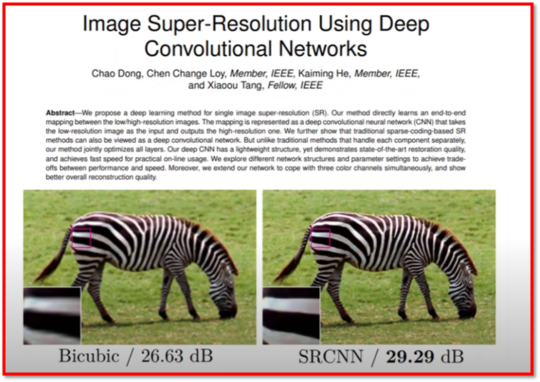
SRCNN(Super-Resolution Convolutional Neural Network), which is designed to increase the resolution of images by learning from high-quality image datasets.
- A notable example is
15.3 Upscaling
Nearest Neighbor Upscaling and Bicubic Upscaling are two common methods used to increase the resolution of digital images. These methods aim to enlarge an image by filling in extra pixels between existing ones, but they do so in different ways, which leads to different visual results.
15.3.1 Nearest neighbour
Nearest Neighbor Upscaling is the simplest and fastest method for enlarging an image.
Here’s how it works:
- Process: In nearest neighbor upscaling, each pixel in the original image is simply duplicated or expanded to fill the larger image grid. When a new pixel is needed, the algorithm looks for the nearest pixel in the original image and copies its value to the new location.
Result: This results in an enlarged image with sharp, blocky edges, as there is no interpolation or averaging of pixel values. Essentially, it makes the pixels appear larger, giving the image a pixelated or “blocky” appearance. This method is quick but often produces low-quality results, especially if the image is scaled up by a significant factor.
Usage: Nearest neighbor upscaling is often used in scenarios where maintaining the exact colour of pixels is more important than producing a smooth result, such as in pixel art or low-resolution graphics.
15.3.2 Bicubic
Bicubic Upscaling is a more advanced technique that produces smoother and higher-quality results compared to nearest neighbor.
Here’s how it works:
- Process: Bicubic upscaling works by considering the weighted average of the 16 closest pixels surrounding the new pixel location (4x4 grid). It uses a cubic interpolation function to estimate the colour of each new pixel by calculating it as a smooth transition between neighboring pixels. The algorithm not only looks at the nearest pixel but also considers the gradient of colour changes in the surrounding area to create a smoother transition.
Result: The bicubic method results in a much smoother and less blocky image compared to nearest neighbor. Edges and gradients between colors are blended more naturally, which reduces visible artifacts like sharp pixel edges. This is particularly useful when enlarging images with fine details.
Usage: Bicubic upscaling is commonly used in photo editing software, video processing, and any application where preserving image quality during resizing is important. It is slower than nearest neighbor due to the additional calculations but provides much better visual results.
15.3.3 Comparison
Nearest Neighbour: Fast, simple, but produces blocky or pixelated images, often used for simple or retro graphics. Bicubic: Slower but results in smoother images with less visible artifacts, preferred for high-quality image resizing.
15.3.4 Data Processing Inequality
In information theory, there is a concept called data processing inequality. It states that whatever way you process data, you cannot add information that is not already there. For example if we have some information X which can be summarised by Y which in turn can be summarised by Y’ then you cannot use Y’ to perfectly reconstruct X≥ This implies that missing data cannot be recovered by further processing.

Does that mean superresolution is theoretically impossible?
15.4 Machine Learning
Machine learning is a subfield of artificial intelligence, which is broadly defined as the capability of a machine to imitate intelligent human behaviour. Artificial intelligence systems are used to perform complex tasks in a way that is similar to how humans solve problems.

15.4.1 Supervised Learning
Supervised learning is a type of machine learning where a model is trained using labeled data. In this approach, the algorithm is provided with input-output pairs, meaning it has access to both the input data (features) and the corresponding correct output (labels). The goal of the supervised learning algorithm is to learn a function that maps the input to the correct output by minimizing the difference between its predictions and the actual labels.
The learning process involves:
Training Phase: The model is trained on a dataset that consists of input-output pairs. The algorithm makes predictions and adjusts itself based on errors through optimization techniques like gradient descent.
Prediction Phase: Once the model is trained, it can be used to predict outputs for new, unseen inputs.
Examples of supervised learning tasks include:
Classification: Predicting categorical labels (e.g., spam vs. non-spam emails).
- The outputs fall under a finite set of possible outcomes. Many situations have only two possible outcomes. This is called binary classification. There are also two other common types of classification: multi-class classification and multi-label classification. Multi-class classification has the same idea behind binary classification, except instead of two possible outcomes, there are three or more.

Regression: Predicting continuous values (e.g., predicting house prices). - The outputs are quantities that can be flexibly determined based on the inputs of the model rather than being confined to a set of possible labels.

In summary, supervised learning relies on labeled data to learn a function that maps an input to an output based on example input-output pairs.
15.4.1.1 Understanding how images work with Machine Learning
- An image is made of “pixels” as shown in the Figure below. In a black-and-white image each pixel is represented by a number ranging from 0 to 255. Most images today use 24-bit colour or higher. An RGB colour image means the colour in a pixel is the combination of Red, Green and Blue, each of the colors ranging from 0 to 255.
- Therefore, as we know images are simply large arrays with multiply dimensions based upon the colour space the image is represented in.
- Since images are simply arrays, we can therefore feed them through neural networks without any modification as seen below where we would learn to output the number
6given the image of a handwrittensix.
- An image 800 pixel wide, 600 pixels high has 800 x 600 = 480,000 pixels = 0.48 megapixels
- An image with a resolution of 1024×768 is a grid with 1,024 columns and 768 rows, which therefore contains 1,024 × 768 = 0.78 megapixels
Using this naive approach to machine learning we would need to construct the input layer of our model to be the same size as the total number of pixels in the image. This becomes a performance issue, when the resolution of images increases.
15.4.2 SRCNN
Now that we understand how nueral networks can process images as input, we can therefore, apply this notation of learning from data to the problem of Upscaling. A popular approach for doing so is called Image Super-Resolution Using Deep Convolutional Networks (SRCNN). This paper can be found at the following link SRCNN
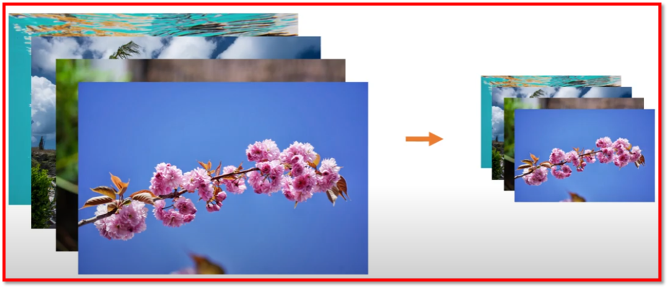
As before, there is the requirement of a dataset, in this case since we are interested in image upscaling we require an image dataset. A popular approach is therefore to have a dataset of low resolution images as well as their high resoloution counterpart. We can then train our model to predict high dimensional images from their lower dimensional counterpart.
There are number of famous image datasets that were created to help facilictate machine learning research and images, namely;
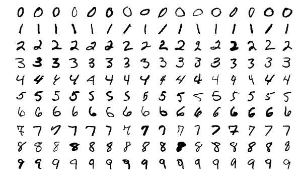
MNIST MNIST is a large dataset of handwritten digits used for training various image processing systems. It was created by Yann LeCun and others in 1998 and has since become one of the most well-known datasets for machine learning and deep learning tasks, especially in the field of image classification.
ImageNet ImageNet is a much larger and more diverse dataset used primarily for visual object recognition tasks. It was created as part of a large visual database project at Stanford University, led by Fei-Fei Li, and has been central to many advancements in deep learning and computer vision

Both datasets have been pivotal in advancing machine learning and deep learning, but ImageNet, in particular, is credited with driving much of the progress in deep neural networks, especially convolutional neural networks (CNNs).
15.4.2.1 Convolutional Machine Learning
The other aspect which is utilised by SRCNN paper is the idea of a convolution.
A Convolutional Neural Network (CNN) is a type of deep learning model designed primarily for tasks involving visual data, such as image classification, object detection, and image segmentation. CNNs have been highly successful in computer vision tasks due to their ability to automatically learn spatial hierarchies of features through convolution operations.
15.4.2.1.1 Key Components of a CNN:
Convolutional Layers:
Purpose: These layers are the core building blocks of a CNN. They apply convolution operations to the input data, enabling the network to automatically learn features like edges, textures, and shapes from images.
Operation: A convolution layer consists of multiple filters (also called kernels), which slide over the input image to extract features. Each filter learns to detect specific patterns in the image, such as edges, corners, or textures. Speifically, the convolution process involves sliding the kernel over the image and performing element-wise multiplication and summation for each position. The following equation corresponds to this process for a 3x3 kernel where \(k\) is the kernel element at \((m,n)\) and \(p\) is the image element at \((i+m-2,j+n-2)\). \[ \text{Output}(i, j) = \sum_{m=1}^{3} \sum_{n=1}^{3} k_{m,n} \cdot p_{i+m-2, j+n-2} \]
Output: The result of applying a filter is a feature map, which highlights where certain patterns appear in the input image.
To get a better understanding on how kernels affect images vist the following link Kernel Playground
Activation Function (usually ReLU):
- Purpose: After each convolution operation, an activation function is applied to introduce non-linearity into the model, allowing it to learn more complex patterns.
- Common Activation Function: ReLU (Rectified Linear Unit) is the most commonly used activation function in CNNs. It replaces all negative values with zero, making the network computationally efficient and helping with the vanishing gradient problem.
Pooling Layers (Subsampling/Downsampling):
- Purpose: Pooling layers reduce the spatial dimensions (width and height) of feature maps, decreasing computational cost and helping prevent overfitting.
-
Types:
- Max Pooling: The most common pooling method, where only the maximum value in each small region (like a 2x2 block) is retained, preserving the most significant features.
- Average Pooling: Takes the average of the values in each small region, though it is less commonly used in modern CNNs.
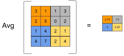
- Effect: Pooling layers allow the network to focus on the most important features and reduce the number of parameters.
Fully Connected Layers (Dense Layers):
- Purpose: After several convolutional and pooling layers, the output is flattened into a 1D vector, which is then fed into one or more fully connected layers. These layers serve the purpose of combining all the learned features to make predictions.
- Operation: Each neuron in the fully connected layer is connected to every neuron in the previous layer, as in a traditional neural network.
Output Layer:
- Purpose: The final fully connected layer produces the output, which could be a classification (for example, identifying objects in an image) or another task-specific result (e.g., object detection or segmentation).
- Activation Functions: The output layer typically uses a softmax function for multi-class classification tasks, as it converts the raw outputs into a probability distribution over classes. For binary classification, sigmoid activation is often used.
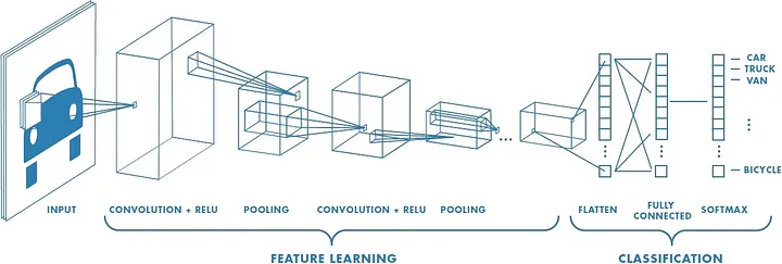
15.4.2.1.2 Structure of a Typical CNN:
A typical CNN architecture involves stacking layers in the following order:
- Input Layer: Takes in an image (e.g., a 2D image for grayscale or 3D for colour images with RGB channels).
- Convolution + Activation Layers: Several convolution layers to extract hierarchical features, each followed by ReLU activation.
- Pooling Layers: Applied after groups of convolution layers to downsample the feature maps.
- Fully Connected Layers: Once the features have been extracted and reduced in size, the final layers are fully connected, leading to a final output prediction.
- Output Layer: Outputs predictions, such as class labels or object locations.
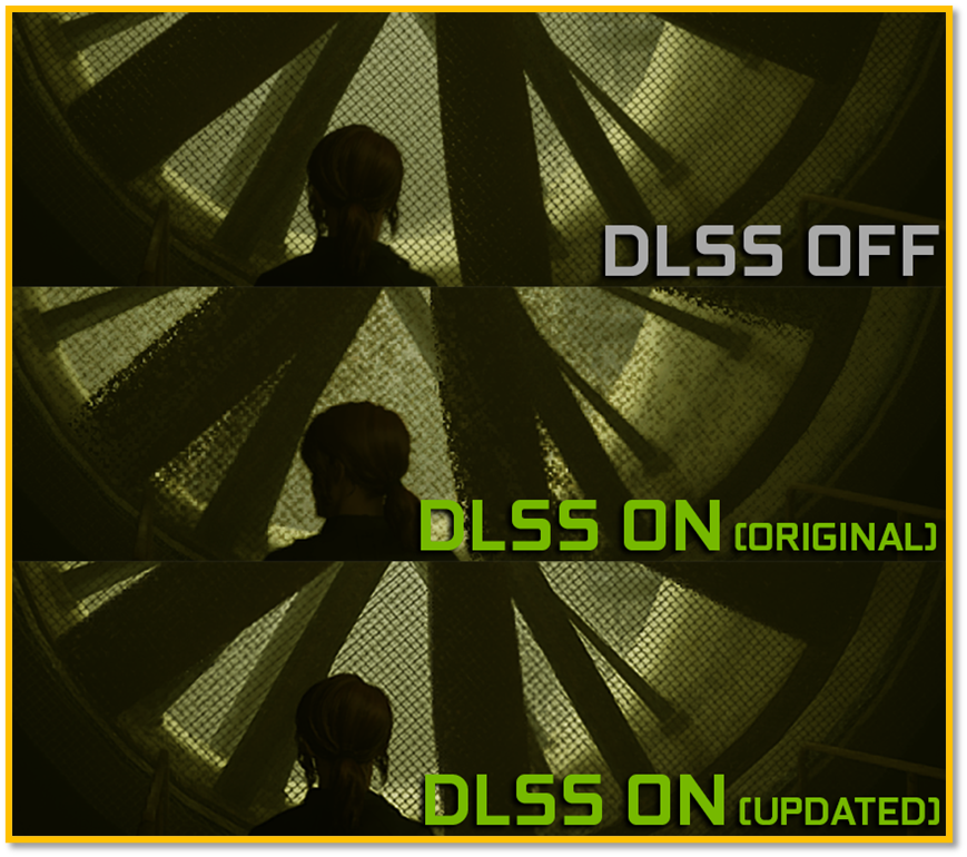
15.4.3 DLSS
DLSS, or Deep Learning Super Sampling, is a technology developed by NVIDIA that uses artificial intelligence and machine learning to enhance graphics rendering in real-time video games. It is specifically designed to improve performance by generating high-resolution images from lower-resolution inputs. DLSS uses a neural network to upscale the images, allowing games to run at higher frame rates without compromising visual quality. It does this by leveraging NVIDIA’s Tensor Cores on RTX GPUs, which are optimized for AI-based tasks. The technology behind DLSS is closely related to a broader class of neural networks called autoencoders, which are often used in tasks like image compression and reconstruction. DLSS’s ability to upscale low-resolution images to high resolution mirrors the compression and reconstruction processes of autoencoders.
15.4.3.1 Auto-Encoders
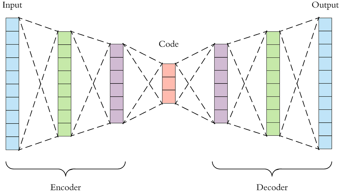
An autoencoder is a type of neural network used for unsupervised learning, primarily for the purposes of dimensionality reduction or feature extraction. Its goal is to learn a compressed representation of input data in a way that allows it to be reconstructed as closely as possible to the original.
- Encoder:
The encoder maps the input data into a lower-dimensional space, called the latent space or bottleneck. This compressed representation is usually smaller than the original input, capturing the most essential features.
- Decoder:
The decoder takes the compressed representation from the encoder and reconstructs it back into the original input space. The goal is for the decoder to reproduce the input data as closely as possible.
15.4.3.1.1 Training Process
- Autoencoders are trained using a method called reconstruction loss, often mean squared error (MSE).
- During training, the network adjusts its parameters to minimize the difference between the input and the reconstructed output.
- Because the encoder learns to compress and the decoder learns to decompress the data, the network becomes efficient at finding a compact representation that preserves the key features.
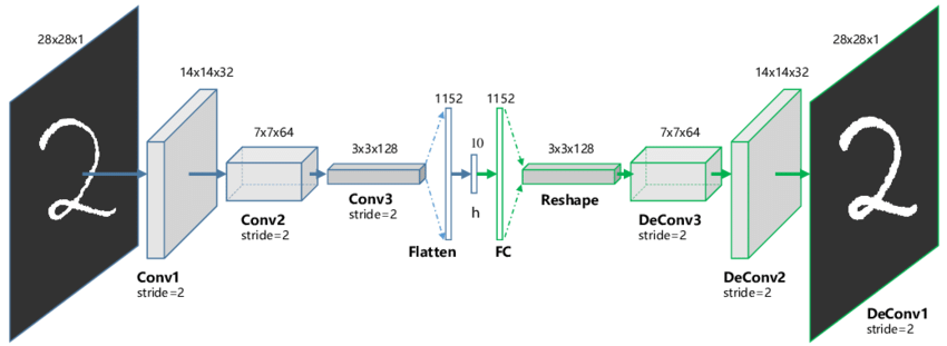
15.4.3.2 Convolutional Auto-Encoders
A convolutional autoencoder has the same fundamental structure as a standard autoencoder—comprising an encoder and a decoder—but it incorporates convolutional layers instead of fully connected layers.
15.4.3.2.1 CAE Training Process
- Like standard autoencoders, CAEs are trained to minimize a reconstruction loss, which measures the difference between the input image and its reconstructed output.
- The loss function often used is the mean squared error (MSE), but other measures like binary cross-entropy can also be applied depending on the data and task.
15.4.3.3 SSI
The Structural Similarity Index (SSIM) is a perceptual metric used to measure the similarity between two images. Unlike traditional metrics like Mean Squared Error (MSE) or Peak Signal-to-Noise Ratio (PSNR), which primarily assess pixel-by-pixel differences, SSIM is designed to evaluate the visual quality of an image by considering structural information that is important to human perception. It was introduced by Zhou Wang and colleagues in 2004. The SSIM index compares the structural information between two images by analyzing the following three components:
Luminance: Compares the brightness (intensity) between two images.
Contrast: Measures the difference in contrast between two images.
Structure: Analyzes the structural similarity (such as edges and textures) between the two images. These components are combined to provide a single SSIM value, which ranges from -1 to 1:
1 means the images are identical.
0 indicates no similarity
Negative values may occur when images are structurally different.
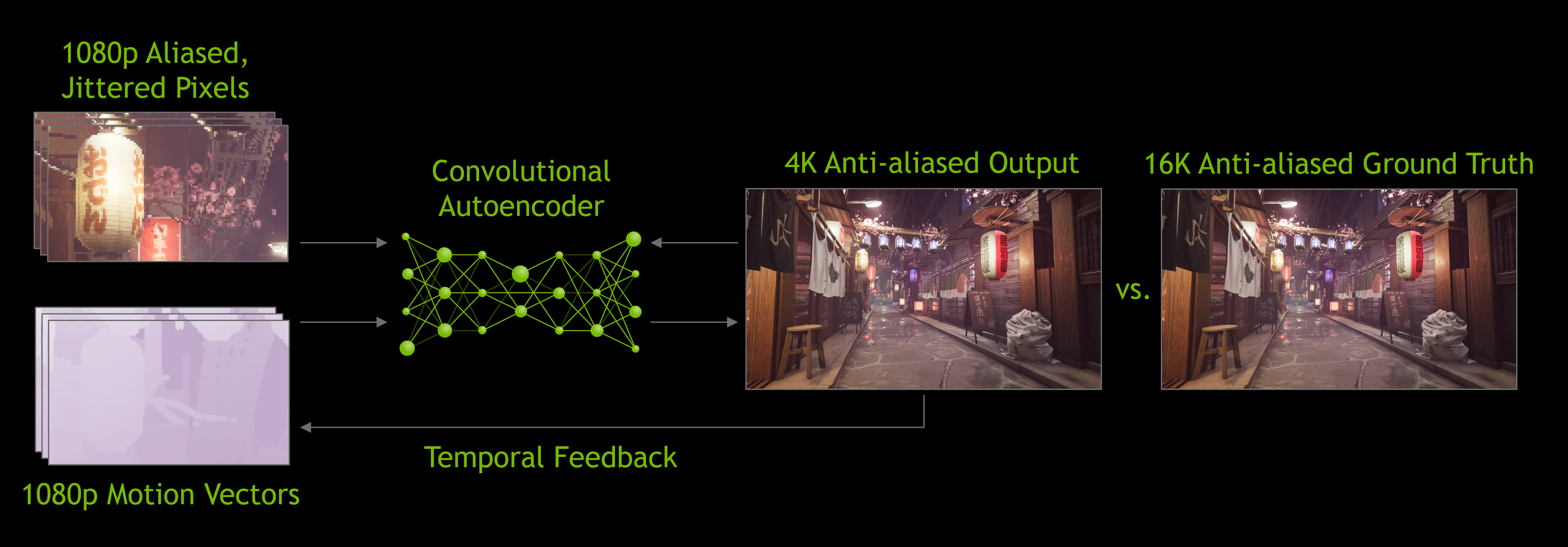
15.4.3.4 What makes DLSS different
Unlike a simple autoencoder that aims to reproduce an input as accurately as possible, DLSS incorporates additional data, like previous frames, to predict and reconstruct a higher-resolution version that looks even better than the input. This makes it more specialized for real-time graphics enhancement, but the underlying principles are similar.
15.4.3.4.1 Results
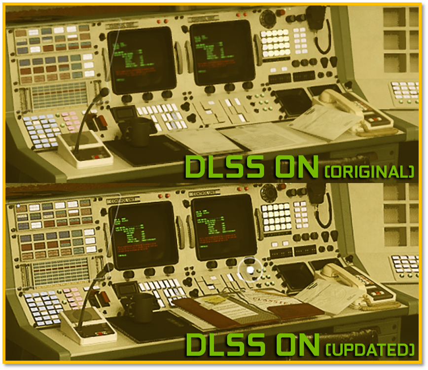
Older games were often designed for lower-resolution screens, with textures that matched the technical limitations of the hardware at the time. As screen resolutions and display technologies have advanced, these older textures can appear blurry or pixelated when played on modern displays. Texture upscaling using machine learning is a process where machine learning models are used to enhance and increase the resolution of textures in older video games, making them look sharper and more detailed. For example, fan projects and some official remasters of older games like Final Fantasy, Resident Evil, or The Legend of Zelda have used AI models to upscale textures, bringing new life to beloved titles.
15.5 Photogrammetry
Photogrammetry is a technique in computer graphics that involves capturing and analyzing images of real-world objects to create precise 3D models and digital representations.
This process involves taking multiple photographs of an object, structure, or environment from different angles and then using specialized software to analyze these photos and generate a detailed 3D model.

15.5.1 Applications in Computer Graphics
- Video Games: Photogrammetry is used to create realistic in-game assets and environments. By scanning real-world objects, game developers can generate highly detailed textures and models, reducing the time and effort needed for manual modeling.
Visual Effects (VFX): In film and TV production, photogrammetry is used to create digital doubles of actors, props, or locations, which can be seamlessly integrated into visual effects shots.
Architectural Visualization: It enables accurate digital reproductions of buildings and archaeological sites for historical preservation, virtual tours, and construction planning.
15.6 Neural Radiance Fields
Neural Radiance Fields (NeRFs) are a method for synthesizing novel views of complex 3D scenes using a sparse set of 2D images as input. NeRFs use a neural network to model the radiance field of a scene, which allows the generation of highly detailed and realistic 3D reconstructions from various angles.
15.6.1 Radiance Field
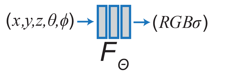
A Radiance Field is a mathematical representation that describes the light properties of a 3D scene. It is expressed as a 5D vector-valued function that has the following characteristics:
-
Input:
- A 3D location 𝑥 = (𝑥,𝑦,𝑧) : This represents a point in space.
- A 2D viewing direction (𝜃,𝜙) : This specifies the direction from which the scene is observed, typically defined using spherical coordinates.
-
Output:
- Emitted colour 𝑐 = (𝑟,𝑔,𝑏) : This defines the colour of the point when viewed from the given direction.
- Volume density 𝛼 : This represents the opacity or density of the point, determining how much light is absorbed or scattered at that location.
In essence, the radiance field describes how light radiates from every point in the scene when viewed from different angles. This makes it suitable for reconstructing complex visual details from different perspectives.
15.6.2 Process
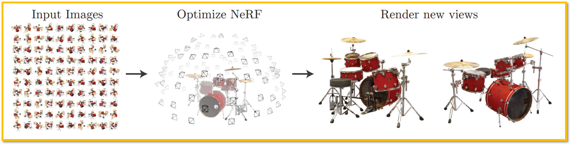
Neural Radiance Fields (NeRFs) use this concept to generate realistic 3D scenes from a sparse set of 2D input images. Here’s a breakdown of how the process works:
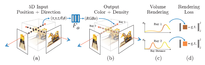
Input Views: In (a) NeRFs start with a sparse set of input views, which are 2D images of a scene captured from different angles. Each input image provides partial information about the scene’s appearance and structure.
Optimization of the Scene Function: The NeRF model learns a continuous function that maps each 3D location and viewing direction to its corresponding colour and volume density in (b). This is achieved through a neural network that is trained using the input images, optimizing to minimize the difference between the observed and predicted images in (d).
Rendering Novel Views: After training, NeRFs can render new views of the scene from arbitrary viewpoints. This allows for the generation of photorealistic images that were not part of the initial input set. Essentially, NeRFs can synthesize how the scene would look from angles that were never directly captured in the input images.
By using a radiance field, NeRFs encode the complex geometry and lighting interactions in a scene, which enables them to produce highly detailed and accurate reconstructions. This makes NeRFs a powerful tool for applications like virtual reality, 3D scene reconstruction, and visual effects in movies and video games.
15.6.3 Use Cases
Neural Radiance Fields (NeRFs) have a range of applications in computer graphics, computer vision, and 3D modeling due to their ability to reconstruct detailed 3D scenes from 2D images. This is valuable for creating detailed virtual environments without needing extensive 3D scanning hardware.