13 Ray Tracing
13.1 Introduction

So far, we have been using rasterization to render 3D scenes. Rasterization is a technique that projects 3D objects onto a 2D plane. It is a fast and efficient way to render 3D scenes, but it has some limitations. For example, rasterization does not handle reflections, refractions, and shadows very well. This is because, to colour a pixel, a rasterizer only needs to know the colour of the object at that pixel. In reality, the colours we see through our eyes are a result of complex interactions between light and surfaces.
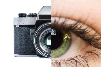
When we look at an object, light rays from the object enter our eyes. Our eyes focus these rays onto the retina, which then sends signals to the brain. The brain processes these signals and we perceive the object. Cameras work in a similar way. They focus light rays onto a sensor, which then captures the image.
The notion of light rays from a light source bouncing off objects and entering our eyes is the basis of ray tracing. Ray tracing is a rendering technique that simulates the way light rays interact with objects in a scene. It traces the path of light rays from the camera to the objects in the scene, and calculates the colour of each pixel based on the interactions between the light rays and the objects.
13.2 The Physics of Light Transport
To understand the principles of ray tracing, it’s important to understand the physics of light transport. In this case, the specific field of study of interest is called “radiometry”, which deals with the measurement of electromagnetic radiation, including visible light, and let’s us formalise the idea of a “light ray”.
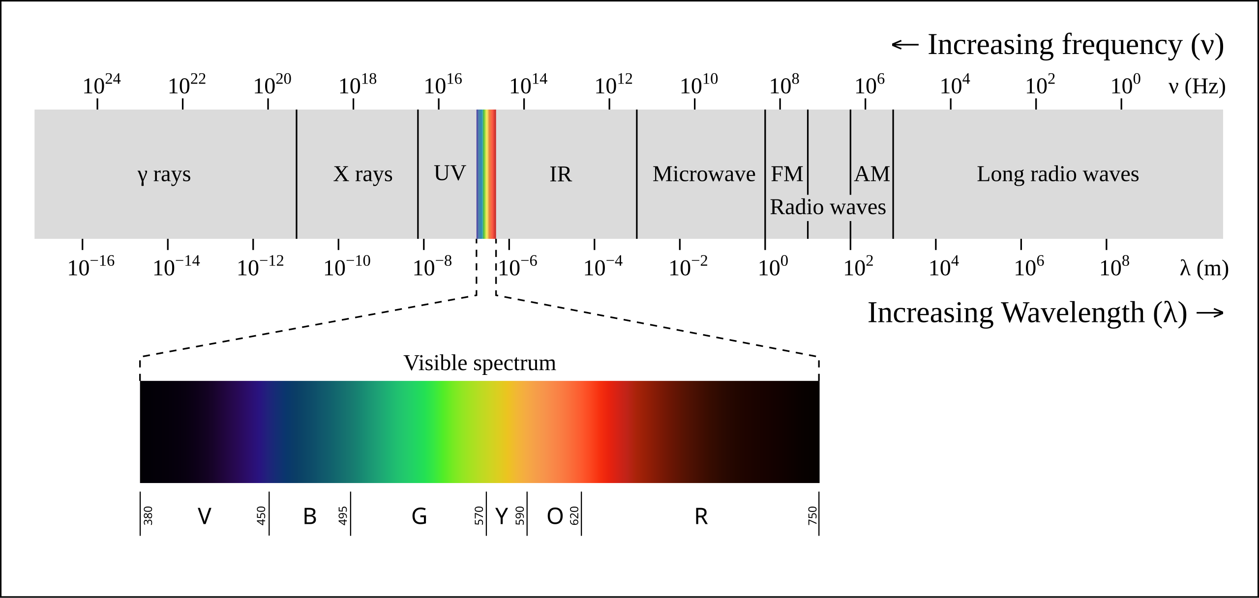
Light rays are the basic unit of light transport. Technically, light rays are not physical entities, but rather a mathematical abstraction that helps us model the behaviour of light. In reality, light, or in this case, visiblie light, is an electromagnetic wave or a stream of photons that carries energy. For the purposes of ray tracing, we can simplify this complex behaviour with the following assumptions:
- Light travels in straight lines. This is known as the principle of rectilinear propagation. In reality, light can bend or refract when it passes through different mediums.
- Light interacts with surfaces in a predictable way. When light hits a surface, it can be absorbed, reflected, or refracted.
- Light does not lose energy as it travels.
13.2.1 Formalising The Light Model
With these assumptions in mind, we can formalise the light transport model used in ray tracing. To fully define what we mean by a ray of light, we need to define the following terms:
13.2.1.1 Radiant Energy
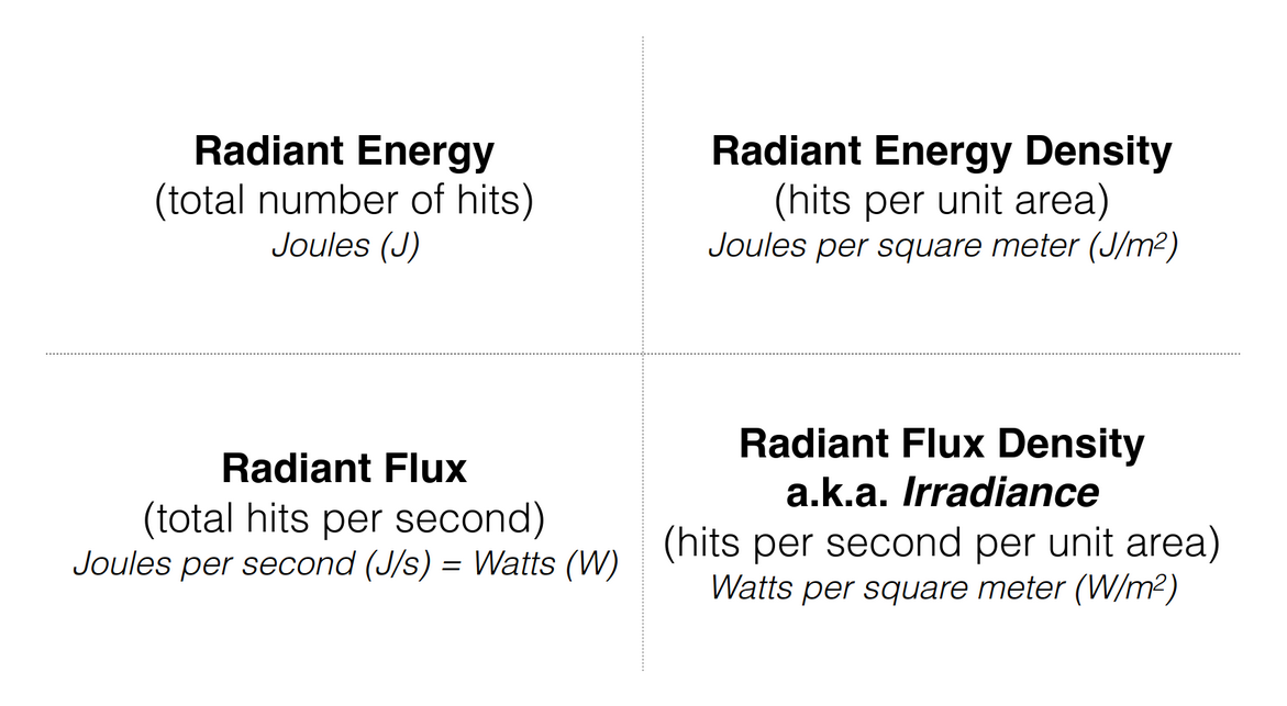
The radiant energy of a surface is given by the total number of light rays that hit the surface. This is measured in Joules/J. Intuitively, the brighter the surface, the more radiant energy it has.
13.2.1.2 Radient Flux
The radiant flux is the rate at which radiant energy is transferred through a surface. This is measured in Watts/W or J/s, Joules per second.
13.2.1.3 Radiant Energy Density
The radiant energy density is the amount of radiant energy per unit area. This is measured in Joules per square meter or J/m^2. If the radiant energy density is high, the surface will appear brighter, and vice versa.
13.2.1.4 Irradiance
The irradiance is the radiant flux incident on a surface per unit area. This is measured in Watts per square meter or W/m^2.
The irradiance is a key concept in ray tracing, as it determines the amount of light energy that a surface receives from the light sources in the scene. Irradiance is independent of the viewing angle, and is a measure of the total amount of light energy that hits a surface. Therefore, it is a key factor in determining the brightness of a surface. However, irradiance alone is not enough to determine the colour of a surface. To calculate the colour of a surface, we need to consider the reflectance properties of the surface, and therefore, we need to know where the light rays are coming from and where they are going.
13.2.1.5 Radiance
By associating a direction with the irradiance, we get the concept of radiance. Formally, radiance is the radiant flux per unit solid angle per unit area perpendicular to the direction of the light. We will not delve into the mathematical details of radiance here, but it is important to understand that radiance is a measure of the brightness of a surface in a particular direction. Radiance is the key concept in ray tracing, when we refer to a “ray of light”, we are referring to the radiance. We denote radiance as L.
The colour of a surface that we perceived is determined by the radiance, therefore term radiance and colour are closely related, but not the same. The colour we preceive is the result of surfaces absorbing light of certain wavelengths and reflecting others. For the rest of this article, we will use these terms interchangeably, but it is important to understand the distinctions between them.
13.2.1.6 Incident and Exitant Rays
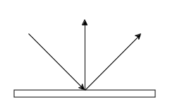
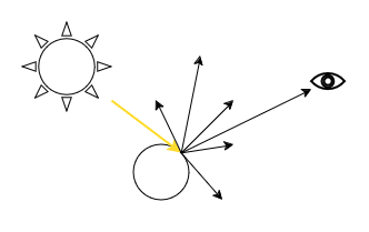
A ray of light can be divided into two parts: the incident ray and the exitant ray. The incident ray is the ray of light that hits a surface, while the exitant ray is the ray of light that leaves the surface. The exitant ray can be further divided into reflected and refracted rays, depending on the surface properties. Reflected rays are always symmetric to the incident rays about the normal to the surface, while refracted rays are bent in more unpredictable ways, we will delve into this in more detail later. In general, the reflected ray is not always equal to the incident ray, as some energy is absorbed by the surface.
13.3 The Rendering Equation
The rendering equation is arguably the most important equation in computer graphics. It describes the light transport in a scene and is the foundation of ray tracing. The rendering equation was first introduced by James Kajiya in 1986, and it has since become the cornerstone of modern rendering algorithms.
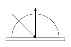
To establish the rendering equation, we need to first consider the irradiance at a point on a surface. Mathematically we can describe this as:
\[ E(p) = \int L(p, \omega) * cos(\theta) d\omega \]
Where: - \(E(p)\) is the irradiance at point p - \(L(p, \omega)\) is the radiance at point p in direction ω, and - \(\theta\) is the angle between the normal to the surface at point p and the direction ω.
Here, the integral is over the hemisphere of directions around the point p. Intuitively, this equation states that the irradiance at a point is the sum of the radiance from all directions, weighted by the cosine of the angle between the normal and the direction. Once the irradiance at a point is known, in other words, we accounted for all the incoming light rays, we can calculate the colour of the surface using the reflectance properties of the surface, i.e., the outgoing light rays. The outgoing light rays are determined by the surface properties, such as the material and the geometry of the surface. We model these properties using the Bidirectional Reflectance Distribution Function (BRDF), which describes how light is reflected off a surface in different directions. The BRDF is typically expressed as:
\[ f(p, \omega_i, \omega_o) \]
Where: - \(p\) is the point on the surface - \(\omega_i\) is the incident direction - \(\omega_o\) is the outgoing direction of interest
We will discuss the BRDF in more detail later, but for now, it is important to understand that the BRDF is a key component of the rendering equation, as it determines how light is reflected off a surface.
13.3.1 The Equation
The rendering equation can be formally stated as:
\[ L_o(p, \omega_o) = L_e(p, \omega_o) + \int f(p, \omega_i, \omega_o) L_i(p, \omega_i) cos(\theta_i) d\omega_i \]
Where: - \(L_o(p, \omega_o)\) is the radiance leaving point p in direction \(\omega_o\) - \(L_e(p, \omega_o)\) is the emitted radiance at point p in direction \(\omega_o\) - \(f(p, \omega_i, \omega_o)\) is the BRDF of the surface at point p - \(L_i(p, \omega_i)\) is the radiance incident on point p from direction \(\omega_i\) - \(\theta_i\) is the angle between the normal to the surface at point p and the direction \(\omega_i\)
The rendering equation states that the radiance leaving a point in a particular direction is the sum of the emitted radiance in that direction and the reflected radiance from all directions weighted by the BRDF and the cosine of the angle between the normal and the direction. In other words, the rendering equation describes how light is transported in a scene, taking into account the interactions between light rays and surfaces.
Note that the rendering equation is defined recursively, as the reflected radiance term itself depends on the radiance incident on the surface, which in turn depends on the radiance leaving other points in the scene. This recursive nature of the rendering equation makes allows us to model complex light transport phenomena such as reflections, refractions, and shadows, which is not possible with rasterization, but it also makes solving the rendering equation computationally expensive.
13.3.2 BRDF
The Bidirectional Reflectance Distribution Function (BRDF) is a key component of the rendering equation. The BRDF describes how light is reflected off a surface in different directions. As previously mentioned, light rays are always reflected symmetrically about the normal to the surface. However, the surface is not always a perfect mirror, i.e. it does not reflect all the light in a single direction, and the direction of reflection can be unpredictable.
To model such unpredictable reflections, we use the BRDF. The BRDF is a probability distribution function that describes how light is reflected off a surface in different directions: instead of modelling the exact path of each reflected light ray, which can be extremely computationally expensive, we model the probability of a light ray being reflected in a particular direction of interest. Therefore, given the definition of the BRDF:
\[ f(p, \omega_i, \omega_o) \]
The BRDF gives the probability that a light ray incident on point \(p\) from direction \(\omega_i\) will be reflected in direction \(\omega_o\), or more intuitively, it gives the proportion of light reflected in direction \(\omega_o\) for a given incident direction ω_i. We call the phenomenon of light being reflected in different directions “scattering”, and the BRDF captures this scattering behaviour.
13.3.2.1 Example BRDFs
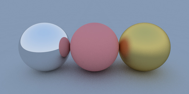
- Ideal Specular Reflection: In this case, the BRDF is a Dirac delta function, which means that all the light is reflected in a single direction. This is the case for perfect mirrors.
- Ideal Diffuse Reflection: In this case, the BRDF is constant, which means that light is reflected uniformly in all directions. This is the case for matte surfaces.
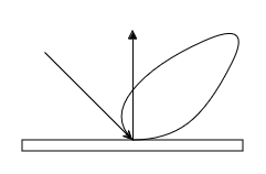
- Glossy Reflection: In this case, the BRDF is a combination of specular and diffuse reflection, which means that light is reflected in a range of directions. This is the case for glossy surfaces.
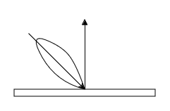
- Retro-Reflection: In this case, the BRDF is peaked in the direction opposite to the incident direction, which means that light is reflected back towards the source. This is the case for retro-reflective surfaces.
13.3.3 Other Scattering Models
The BRDF is a subset of models called Bidirectional Scattering Distribution Functions (BSDFs), which describe how light is scattered in all directions, not just the reflected direction. The BSDF is a more general form of the BRDF, as it includes both reflection and refraction. The BSDF is used to model more complex light transport phenomena such as subsurface scattering, where light penetrates the surface of an object and is scattered inside the material before exiting. Examples of what more general BSDFs can model include:
Subsurface Scattering: Light penetrates the surface of an object and is scattered inside the material before exiting. This is the phenomenon that gives objects like skin, wax, and milk their characteristic appearance.
Refraction: Light changes direction as it passes through different mediums, such as air and glass.
13.4 Ray Tracing
Ray tracing is a rendering technique that simulates the way light rays interact with objects in a scene.
We algorithmically trace the path of light rays from the camera to the objects in the scene, and calculate the colour of each pixel based on the interactions between the light rays and the objects, using the rendering equation.
13.4.1 Forward Ray Tracing
Forward ray tracing is the most basic form of ray tracing. Forward ray tracing is the most basic form of ray tracing. It follows the path of light rays in the real world, and generates an image based on all the rays that eventually reach the camera.
For each light source in the scene, we trace numerous rays from the light source into the scene. There are techinically an infinite number of rays from the light source. But for computability, we typically only sample a finite subset of them.
As the rays intersect with objects in the scene, we calculate the colour and directional information of the rays based on the interactions between the ray and the objects. Note that due to factors such as the complexity of the geometry of the scene, there is no guarantee that a ray will eventually reach the camera, i.e. it will not contribute the final image, meaning all the computation spent on tracing that ray is wasted. To render a final image using forward ray tracing would require a large enough number of rays to be traced such that a sufficient number of rays reach the camera to form a coherent image. This can be computationally expensive, especially for complex scenes.
13.4.2 Reverse Ray Tracing
To address the inefficiency of forward ray tracing, reverse ray tracing was introduced.
In reverse ray tracing, we trace rays of from the camera into the scene, guaranteeing that each ray we trace will contribute to the final image, eliminating the issue of wasted computation inherent in forward ray tracing.
13.4.2.1 Ray Generation
In reverse ray tracing, we start by generating rays from the camera into the scene. Given a camera location, we generate a ray for each pixel in the image plane.
The origin of the ray is the camera location, and the direction of the ray is determined by the position of the pixel on the image plane.
13.4.2.2 Ray Intersection
Once we have generated the rays, we trace them into the scene. We check for intersections between the rays and the objects in the scene. This is not a trivial task, as it involves solving the intersection of a ray with complex geometric objects such as spheres, triangles, and polygons.
The most common method for ray-object intersection is the “ray-object intersection test”, which involves checking if the ray intersects with the bounding box of the object, and then checking if the ray intersects with the actual geometry of the object. Another method is the “ray-triangle intersection test”, which involves checking if the ray intersects with the plane of the triangle, which form the meshes of an object, and then checking if the intersection point lies within the bounds of the triangle using baricentric coordinates. An interested reader can look up the details of these methods.
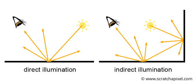
13.4.2.3 Direct Illumination
Once we have determined the intersection point, we can determine if the point is in shadow or not. If the point is in shadow, we do not need to calculate the colour of the point, as it will not be visible in the final image. If the point is not in shadow, we calculate the radiance from the point (the colour) based on the interactions between the light rays and the objects in the scene.
Whether or not a point is in shadow can be determined easily by tracing another ray from the intersection point to the light source. This is called a shadow ray. If the shadow ray intersects with another object before reaching the light source, then the point is in shadow.
This is called direct illumination: determining whether any point is illuminated by a light source directly. This is a simplification of the rendering equation, as it only considers the direct light sources in the scene, and does not account for indirect illumination, i.e. light that is reflected off other surfaces in the scene onto the point of interest.
13.4.2.4 Global Illumination
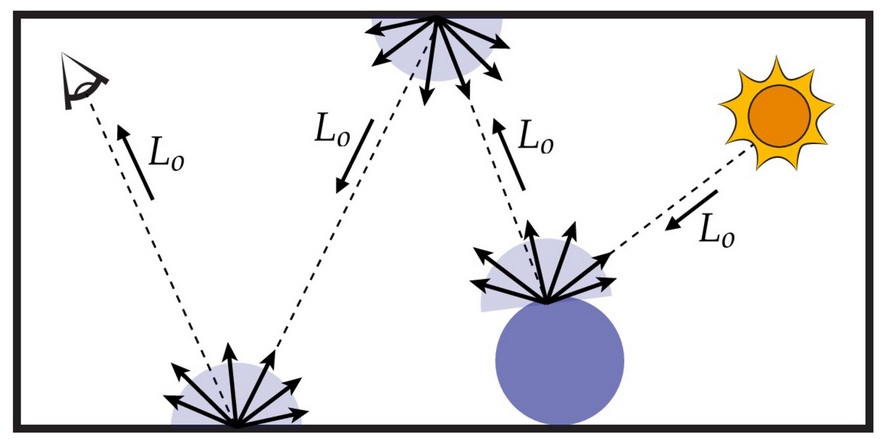
To account for indirect illumination, we need to consider the interactions between light rays and surfaces in the scene. This is also called global illumination (GI).
In GI, we recusively trace rays from the intersection point to other points in the scene, and calculate the irradiance of the point as the sum of all the reflected light rays from other points in the scene, according to the rendering equation. And for every ray we trace from this point, we recursively trace more rays from the new intersection points, and so on. This process continues until a certain termination condition is met, such as a maximum recursion depth or a minimum intensity threshold, i.e. the ray is too dim to contribute to the point.
13.4.2.5 Monte Carlo Ray Tracing
According to the rendering equation, we need to integrate the incoming radiance from all directions to calculate the colour of a point. This is computationally intractable, as it involves tracing an infinite number of rays in all directions. A common approach to solving this problem is Monte Carlo ray tracing, which involves sampling a finite number of rays in random directions and averaging the results to approximate the integral. This is a statistical method that converges to the correct solution as the number of samples increases. Because of the randomness of the sampling, Monte Carlo ray tracing is inherently noisy, and requires a large number of samples to produce a noise-free image. And because we can only sample a finite number of rays at each point of intersection, to get a good approximation of the integral, we need to perform multiple iterations of the ray tracing process.
Monte Carlo ray tracing allows us to simulate the complex phenomena of light transport in a scene. It is the basis of many modern rendering algorithms. However, it is computationally expensive, as it requires a large number of samples to produce a high-quality image and many iterations to approximate to the correct solution, with no gaurentee of convergence and often results in noisy images.
There are many techniques to reduce the noise in Monte Carlo ray tracing, such as importance sampling, path tracing, and denoising algorithms. An interested reader can look up these techniques for more information.
13.4.3 Implementating a Ray Tracer
The complexity of the ray tracing algorithm is beyond the scope of this course, but it is important to understand its connection to the concepts of shaders and GPUs that we’ve discussed in previous lessons. Due to the way the rays are generated, we can closely associate a pixel in the final image with a ray of light. Each ray we trace is independent of the other rays, and can be computed in parallel. This makes ray tracing highly parallelizable, and well-suited for modern graphics hardware such as GPUs. Often ray tracing is implemented using the CUDA or shader programming languages, which are designed for parallel computation. Because fragment shaders in GPUs are designed to compute the colour of each pixel independently, they are well-suited for ray tracing.
A link to the code implementation of ray tracing can be found here.
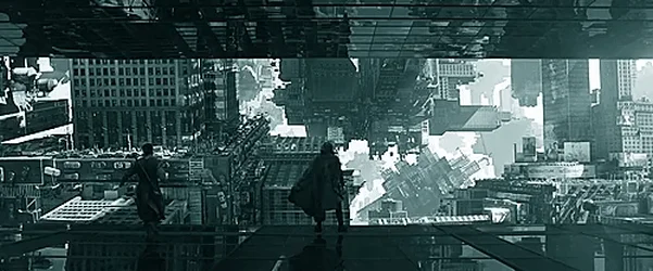
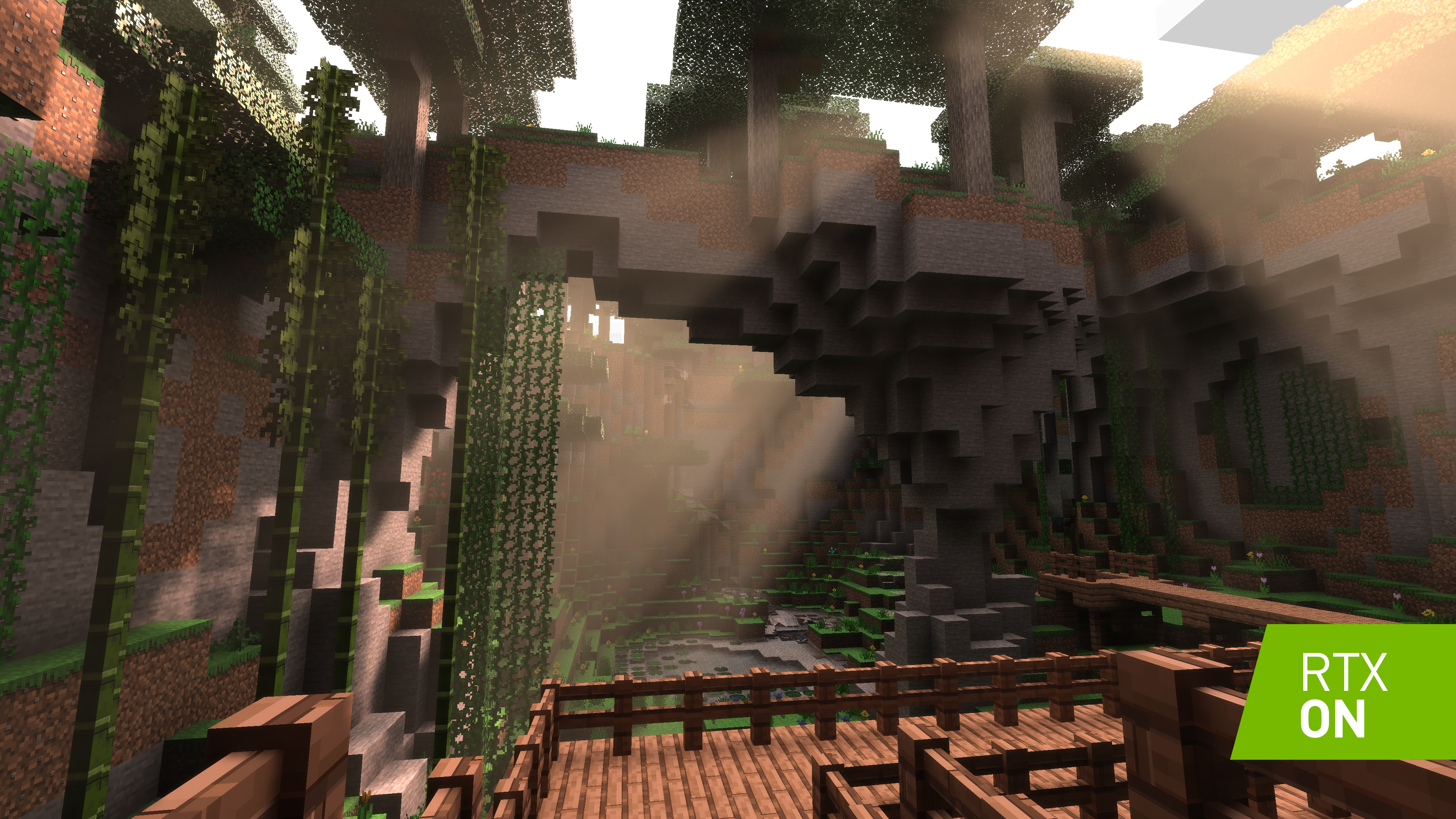
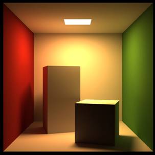
13.5 Ray Tracing in Practice
Ray tracing is most often used in applications where photorealistic rendering is required, such as in movies, video games, and architectural visualization. Here are a few examples and demonstrations of ray tracing in practice: